Speculative Decoding Architecture: Accelerating Enterprise LLM Inference Without Sacrificing Accuracy

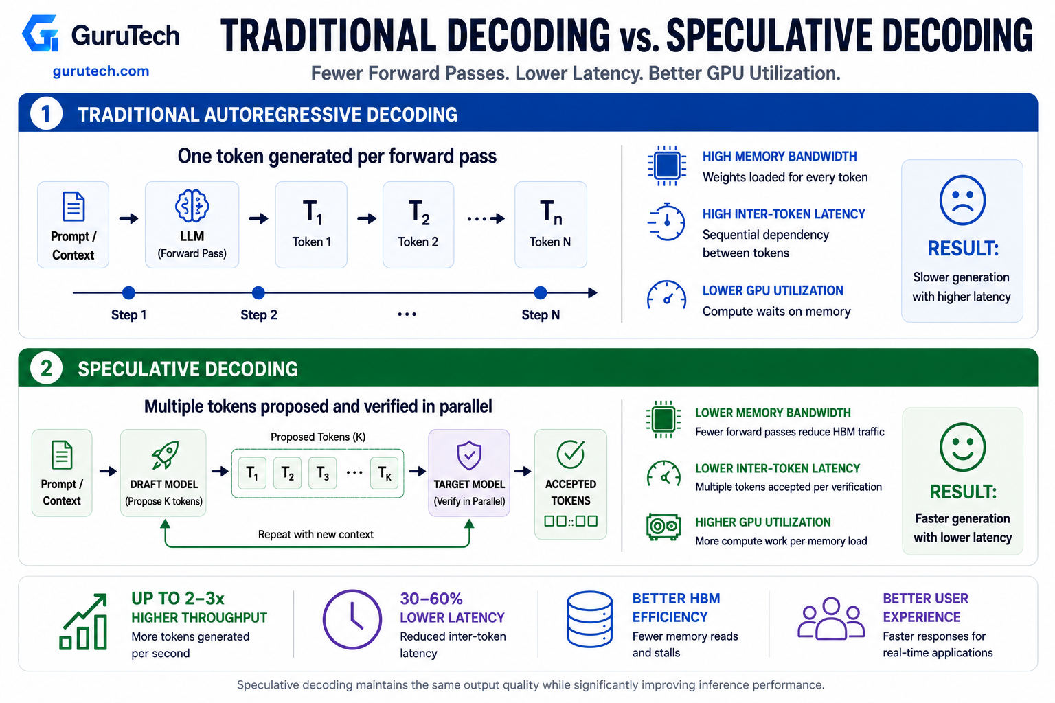
Large language model inference in production environments faces a fundamental constraint that no amount of hardware can fully eliminate. Every token your model generates requires loading billions of parameters from GPU memory, creating a memory bandwidth bottleneck that leaves compute cores underutilized.

Speculative decoding architecture addresses this inefficiency by pairing your target model with a lightweight draft model that proposes multiple candidate tokens, which the target model then verifies in parallel during a single forward pass, reducing overall latency without compromising output quality.

This approach transforms the sequential token-by-token generation process into one where your system can accept multiple tokens per verification step. This directly improves inter-token latency in your deployment.

The architecture works by offloading initial token prediction to a smaller, faster draft mechanism while your target model focuses on verification rather than generation.

When implemented correctly within frameworks like vLLM’s speculative decoding pipeline or SGLang, the technique maintains identical output distributions to standard autoregressive decoding. It collapses multiple sequential memory-bound operations into fewer passes.

Your infrastructure benefits from improved GPU utilization and lower end-user latency. This is particularly important in interactive applications where response time directly impacts user experience.

Memory bandwidth trade-offs and production monitoring strategies are also essential. Whether you’re evaluating EAGLE-3 or multi-token prediction approaches, your deployment decisions will determine whether the technique delivers measurable improvements or introduces unnecessary overhead into your serving infrastructure.

Understanding Latency in Autoregressive Decoding

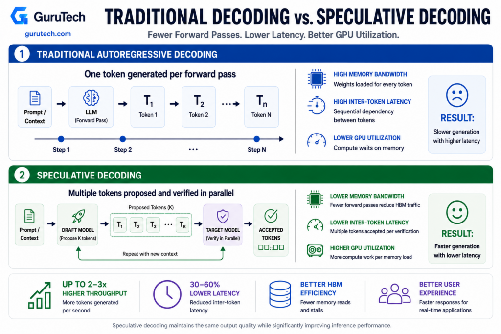
Autoregressive decoding in large language models faces a fundamental bottleneck where memory bandwidth limits throughput more than raw computational power. The sequential nature of token generation forces GPUs to spend most of their time waiting for weight data rather than performing calculations.

Memory-Bound Processing Explained

Your GPU’s compute units sit idle during most of LLM inference because the process is memory-bound rather than compute-bound. Each token generation requires loading billions of parameters from memory, performing a relatively small number of matrix operations, then repeating the cycle.

The ratio of computation to memory access is extremely low in autoregressive decoding. You might have a GPU capable of 300 TFLOPS, yet only 10-15% of that capacity gets utilized during single-token generation.

The remaining capacity waits on memory transfers to complete. This inefficiency compounds with model size.

A 70B parameter model requires moving approximately 140GB of data for each forward pass when using FP16 precision. The actual arithmetic operations complete in microseconds once the data arrives.

The Role of HBM Access

High Bandwidth Memory determines your effective inference speed more than any other hardware specification. Modern GPUs provide 2-3 TB/s of HBM bandwidth, which sounds impressive until you calculate the time needed to load full model weights.

Your memory bandwidth directly caps token generation rate. A simple weight-size-to-bandwidth calculation illustrates the lower bound: moving 140GB across a 2TB/s memory subsystem would take roughly 70ms before computation, caching effects, parallelism, and implementation overhead are considered.

Key HBM constraints you face:

• Weight tensors must transfer from HBM to compute units for each layer.
• Activation values require intermediate storage and retrieval.
• KV cache grows with sequence length, consuming additional bandwidth.
• Batch size increases memory pressure without proportional latency reduction.

Arithmetic Intensity Constraints

Arithmetic intensity measures the ratio of compute operations to memory accesses, expressed as FLOP per byte. Autoregressive decoding exhibits extremely low arithmetic intensity, typically below 1 FLOP/byte for single-token generation.

You need high arithmetic intensity to fully utilize your GPU’s capabilities. Matrix multiplication in the prefill phase achieves 50-100 FLOP/byte because you process many tokens simultaneously.

The decode phase processes one token at a time, resulting in 0.5-2 FLOP/byte. This creates a fundamental mismatch.

Your GPU’s balance point might be 150 FLOP/byte, meaning you would need 150 operations per byte transferred to reach peak efficiency. Autoregressive decoding performs 75-300x fewer operations than optimal.

Batch processing helps but provides diminishing returns. Increasing batch size from 1 to 8 improves arithmetic intensity but doesn’t solve the sequential dependency problem inherent in token-by-token generation.

GPU Memory Stalls

Your GPU cores spend 60-80% of their time stalled during autoregressive decoding, waiting for memory operations to complete. These stalls occur at multiple levels of the memory hierarchy, from L1 cache misses to DRAM access latency.

Pipeline bubbles form when compute units finish their assigned work but cannot proceed because required data hasn’t arrived from HBM. The sequential nature of autoregressive generation prevents you from hiding latency through parallel work scheduling.

Memory bank conflicts add unpredictable delays. When multiple memory requests target the same bank, they serialize rather than execute in parallel.

Your effective bandwidth drops below the theoretical maximum, sometimes by 20-30%.

Integrating with Local LLM Deployment

Your local deployment architecture must account for memory bandwidth limitations when sizing infrastructure. A server with multiple GPUs doesn’t automatically deliver proportional speedup because each model instance still faces the same memory-bound constraints.

Sequential dependencies impose lower bounds on latency and parallelism that architectural changes alone cannot overcome. You need algorithmic improvements like speculative decoding to break through these barriers.

Consider tensor parallelism carefully. Splitting a model across 4 GPUs requires 4x the aggregate memory bandwidth but adds communication overhead.

Your per-token latency may only improve by 2-3x while quadrupling hardware costs.

Practical deployment considerations:

• GPU selection: Prioritize HBM bandwidth over TFLOPS when comparing options.
• Batching strategy: Implement dynamic batching to maximize arithmetic intensity without sacrificing latency.
• Memory allocation: Reserve sufficient VRAM for KV cache growth across long sequences.
• Monitoring: Track memory bandwidth utilization, not just GPU compute percentage.

Design Principles of Speculative Decoding

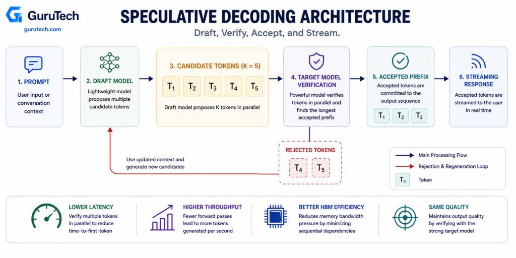
Speculative decoding architecture relies on coordinating two computational stages: a lightweight draft model rapidly proposes token sequences, while the target model verifies these candidates in parallel to maintain output quality identical to standard autoregressive generation.

Draft Model Generation

Your draft model serves as the speculation engine that generates candidate tokens ahead of the main target model. The speedup from speculative decoding heavily depends on your choice of draft model, making this selection critical for performance gains.

The draft model must balance two competing requirements: speed and accuracy. Smaller models generate tokens faster but may produce lower-quality candidates that the target model rejects.

Larger draft models improve acceptance rates but reduce the speed advantage that makes speculative decoding viable. You typically select draft models through one of three approaches:

• Distilled models trained using the target model’s outputs as ground truth
• Quantized versions of the target model itself
• Earlier checkpoints from the same training run

Draft model inference operates autoregressively just like standard generation, but its smaller size means each forward pass completes significantly faster. You configure the draft model to generate between 3 and 12 speculative tokens per iteration, with the optimal number depending on acceptance rate patterns in your specific workload.

Candidate Generation Process

Once you’ve selected a draft model, the candidate generation process begins with the current context. Your draft model extends the input sequence by generating multiple tokens sequentially, building a proposed continuation that the target model will later verify.

The generation process uses standard sampling techniques like temperature scaling, top-k filtering, or nucleus sampling. These parameters control the diversity and confidence of candidate tokens.

Higher temperature values increase exploration but typically lower acceptance rates, while conservative sampling improves verification success at the cost of reduced creativity. Hardware-efficient draft models can provide 111% higher throughput compared to conventional draft architectures by optimizing memory access patterns and computational efficiency.

Parallel Verification Mechanism

Your target model receives all draft tokens simultaneously and processes them in a single forward pass. This parallel verification approach represents the core efficiency gain of speculative decoding, transforming multiple sequential operations into one batched computation.

The verification process computes probability distributions for each position in the draft sequence. Because the target model has already cached key-value pairs from the original prefix, only the speculative tokens incur computational cost during verification.

This selective processing minimizes overhead while ensuring output quality. The target model compares its own probability distribution against the draft model’s predictions for each token position.

For sampling-based decoding, the acceptance decision uses the ratio between target and draft probabilities together with rejection sampling; greedy decoding can use direct token agreement. The system accepts tokens sequentially until it encounters the first rejection or reaches the end of the draft sequence.

Verification Stage	Operation	Computational Cost
Load cached KV pairs	Retrieve stored activations	Minimal memory access
Process draft tokens	Single forward pass	One target model inference
Compute probabilities	Generate distributions	Standard output layer cost
Compare distributions	Token-by-token validation	Negligible arithmetic

Accepted Prefix Workflow

After verification completes, you determine which draft tokens to accept based on the comparison between target and draft probabilities. The acceptance logic implements rejection sampling to maintain mathematical equivalence with standard autoregressive generation.

Your system accepts the longest prefix where every token satisfies the acceptance criterion. If the target model accepts all draft tokens, you’ve successfully generated multiple tokens in a single iteration.

When the target model rejects a token, you discard that token and all subsequent draft predictions. The acceptance rate directly determines your speedup factor.

A 60% acceptance rate on 5 draft tokens means you typically accept 3 tokens per iteration, compared to 1 token in standard generation. This metric varies based on task difficulty, model alignment, and the similarity between draft and target model training.

Upon rejection, the system doesn’t simply discard the problematic token. Instead, the target model samples a corrected token from an adjusted probability distribution that accounts for the draft model’s incorrect prediction.

This correction mechanism ensures the output distribution matches what pure target model generation would produce.

Continuing Inference Steps

After processing the accepted prefix, your inference pipeline updates the context and prepares for the next speculation cycle. The newly accepted tokens become part of the input context for subsequent draft model generation.

You append accepted tokens to the key-value cache, avoiding redundant recomputation of attention activations. This cache update happens regardless of how many tokens were accepted, maintaining efficiency across varying acceptance patterns.

The next iteration begins with the draft model generating new candidates from the updated context. This cyclic process continues until you reach a stopping condition: maximum token limit, end-of-sequence token, or application-specific termination criteria.

Dynamic draft tree approaches adapt the speculation strategy based on recent acceptance patterns. If your system detects consistently low acceptance rates, it may reduce the number of speculative tokens to minimize wasted computation.

Conversely, high acceptance rates justify more aggressive speculation.

Enterprise Pipeline Integration

Integrating speculative decoding into production systems requires coordination across multiple infrastructure components. You need to manage two model artifacts: the target model weights and the draft model (or EAGLE head) parameters.

Heterogeneous architecture designs partition speculative decoding into separate hardware components, with FPGA-based drafting and GPU-based verification exploiting complementary strengths.

Your deployment pipeline must handle:

• Model versioning: Keeping draft and target models synchronized
• Resource allocation: Distributing GPU memory between both models
• Request batching: Grouping inference requests to maximize throughput
• Monitoring instrumentation: Tracking acceptance rates and latency metrics

Frameworks like TensorRT-LLM, vLLM, and SGLang provide native support for speculative decoding, abstracting many implementation details. These platforms handle scheduling, memory management, and the coordination between draft and target model executions.

You should implement feature flags that allow toggling speculative decoding on and off without code changes. This flexibility enables A/B testing and provides a fallback mechanism if acceptance rates drop below profitable thresholds for specific workload patterns.

Evaluating Draft Models Against Target Models

Draft model evaluation determines whether a smaller model can effectively accelerate a target LLM through speculative decoding. The acceptance rate between your draft model and target model directly impacts inference speedup, making compatibility checks and architectural alignment critical before deployment.

Model Compatibility Checks

Your draft model must generate tokens that align closely with your target model’s distribution. The acceptance rate measures how often the target model accepts draft tokens during verification, and research shows this heavily depends on draft model choice.

You should test multiple draft model candidates against your target model using representative workloads. A draft model with strong perplexity scores on standard benchmarks may still perform poorly in speculative decoding if its output distribution diverges from your target model.

Key compatibility factors:

• Model family alignment: Draft models trained from the same architecture family typically achieve higher acceptance rates
• Training data overlap: Shared pretraining data between draft and target improves token prediction alignment
• Domain specialization: Generic draft models experience significant acceptance rate drops with domain-specific targets

Test your draft model across different prompt types and generation lengths. Acceptance rates often vary significantly between short completions and long-form generation tasks.

Tokenizer Alignment Strategies

In the simplest and most widely supported configuration, the draft and target models use the same tokenizer and vocabulary. Tokenizer mismatches cause immediate verification failures because the draft model generates token IDs that the target model cannot interpret.

When tokenizer or vocabulary mappings differ, the serving engine must explicitly support and correctly translate heterogeneous token spaces. Differences in special tokens, whitespace, or Unicode handling can reduce compatibility or require an explicit mapping layer.

You can verify tokenizer compatibility by encoding identical text strings with both models and comparing output token sequences. Any divergence indicates incompatibility that requires resolution before deployment.

Ensuring Architectural Match

Your draft model architecture must produce logits compatible with your target model’s vocabulary and output format. While the draft model can have fewer layers, different hidden dimensions, or reduced attention heads, the final output projection must match.

Architectural mismatches in the vocabulary projection layer prevent proper token verification. Your draft model’s logit output shape must align with the target model’s vocabulary size and token representation scheme.

Compatible architectural variations:

• Reduced transformer layers (e.g., 6 layers vs 32 layers)
• Smaller hidden dimensions and attention heads
• Modified attention mechanisms (MQA, GQA instead of MHA)
• Pruned or distilled versions of the target architecture

You should verify that both models handle the same context length and position encoding scheme. Context window mismatches can cause failures during longer generation sequences.

Acceptance Probability Analysis

The acceptance probability determines your actual inference speedup from speculative decoding. You calculate this by dividing accepted draft tokens by total proposed tokens across your evaluation dataset.

Higher acceptance rates translate directly to greater speedup. Studies with LLaMA-65B and OPT-66B show that draft model latency matters more than raw language modeling capability for overall performance.

You should measure acceptance rates across different generation scenarios:

Scenario Type	Target Acceptance Rate	Impact on Speedup
Greedy decoding	>70%	2-3x speedup
Low temperature sampling	>60%	1.8-2.5x speedup
High temperature sampling	>40%	1.3-1.8x speedup
Domain-specific tasks	>50%	1.5-2x speedup

Your acceptance rate analysis should include variance measurements. Consistent acceptance rates across diverse inputs indicate robust draft model performance.

Multi-Token Verification Techniques

Multi-token verification enables the target model to evaluate multiple candidate tokens simultaneously rather than processing them sequentially. The verification pass examines draft proposals in parallel by computing probability distributions across all positions, then applies acceptance logic to determine which tokens match the target model’s own predictions.

K-Lookahead Methods

K-lookahead defines how many tokens ahead your draft mechanism proposes in each speculation round. You’ll typically configure between 3 to 12 tokens as your lookahead window, though the optimal value depends on your specific model pairing and workload characteristics.

The lookahead length directly impacts your verification efficiency. A larger K value means more tokens verified per pass, but it also increases the computational cost of each verification step and raises the probability that later tokens in the sequence will be rejected.

Your draft model’s accuracy typically degrades with distance from the known prefix, making tokens further in the lookahead window less likely to match target model predictions.

You should tune K based on your observed acceptance rates. If you’re consistently accepting only the first 2-3 tokens from a 10-token draft, you’re wasting verification compute on proposals that get discarded.

Verification Pass Mechanics

Your target model processes the input sequence plus all draft tokens in a single forward pass, leveraging the KV cache to avoid recomputing attention values for the original prefix.

Only the newly speculated tokens incur computational cost during verification, which is why parallel verification provides key efficiency gains compared to sequential generation.

The verification step computes probability distributions at each token position. Your target model generates logits for every position in the draft sequence simultaneously, producing a complete probability distribution that shows what tokens the target model would have selected at each step.

These distributions become the ground truth against which draft proposals are evaluated.

You can optimize verification performance by batching multiple speculation attempts together when serving concurrent requests. The target model’s capacity to process sequences in parallel means verification overhead scales sublinearly with the number of draft tokens.

Acceptance Logic

Your acceptance logic compares the draft model’s proposed probability P(Draft) against the target model’s actual probability P(Target) for each token position. When P(Target) exceeds or meets P(Draft), you accept the token and continue evaluating the next position in the sequence.

The comparison happens sequentially through the draft tokens even though probabilities were computed in parallel. You evaluate the first draft token, and only if accepted do you proceed to evaluate the second token.

This sequential acceptance ensures coherent output that matches what your target model would generate autoregressively.

Acceptance rate measures the percentage of draft tokens your target model validates:

• High acceptance (>70%): Your draft mechanism closely approximates target model behavior
• Moderate acceptance (40-70%): Reasonable speedup with room for improvement
• Low acceptance (<40%): Draft quality issues or mismatched model distributions

Rejection Pathways

When your acceptance logic encounters a token where P(Target) falls below P(Draft), it triggers rejection. You immediately discard that token and all subsequent tokens in the draft sequence, regardless of their individual probabilities.

The verification process then reverts to standard autoregressive generation from the last accepted token position. Your system samples a corrected token from the target model’s probability distribution at the rejection point.

This corrected token becomes part of the verified prefix for the next speculation round. The process maintains output quality by ensuring every token in the final sequence either passed verification or was directly generated by the target model.

You’ll see rejection patterns emerge based on content complexity. Predictable text like common phrases or structured formats typically yields higher acceptance rates, while creative or technical content with less predictable token sequences triggers more frequent rejection pathways.

Illustrative Verification Timelines

Standard autoregressive generation with 200ms per forward pass requires 600ms to produce three tokens through three sequential steps.

Speculative decoding collapses this into a single 250ms verification pass that validates two draft tokens and generates one additional token.

Your timeline breakdown looks like this:

Generation Method	Steps	Time per Step	Total Time	Tokens Generated
Autoregressive	3	200ms	600ms	3
Speculative (2 accepted)	1	250ms	250ms	3

The verification overhead adds 50ms compared to a single autoregressive step, but you generate three tokens instead of one.

Your net speedup reaches 2.4x in this example.

You’ll experience the latency reduction most noticeably in interactive applications.

Instead of watching tokens appear one by one with distinct pauses, users see responses materialize in faster multi-token chunks that create a more fluid experience.

Balancing Memory Bandwidth and Compute Utilization

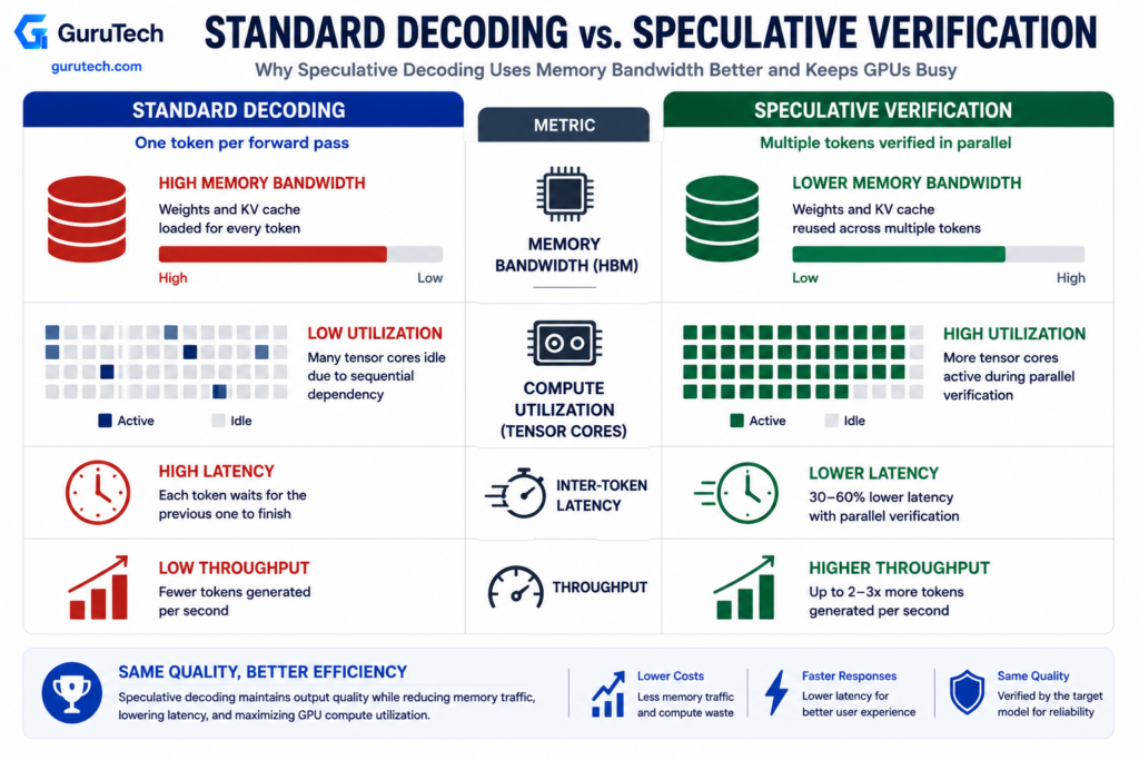
Modern GPUs possess more computational throughput than they can effectively use during standard autoregressive decoding, creating an imbalance where memory bandwidth becomes the dominant bottleneck rather than compute capacity.

Speculative decoding exploits this gap by trading additional compute work for fewer memory-bound operations.

Comparing Bandwidth to Compute

Your GPU’s compute units sit idle during standard token generation because the expensive operation is moving model weights from high-bandwidth memory into on-chip registers.

Each forward pass requires streaming the entire weight matrix from VRAM to compute units, regardless of how many tokens you process simultaneously.

This creates an opportunity for GPU inference optimization.

When you verify multiple draft tokens in parallel, the weight matrix loads from memory exactly once to verify the entire block, converting a memory-bound task into a compute-bound operation.

Your GPU has surplus FLOPs available during single-token generation.

The sequential dependency of autoregressive decoding prevents parallel processing of multiple positions, leaving compute capacity unused.

Speculative decoding fills this gap by processing candidate tokens simultaneously during verification, maximizing utilization of existing computational resources without requiring additional hardware.

Amortized Verification Impact

When you verify four draft tokens simultaneously, you amortize the memory transfer cost across all candidates instead of paying it four separate times.

The verification phase processes all tokens in one forward pass, reducing the number of weight loads from VRAM by the acceptance length.

Your effective throughput increases because each memory operation produces multiple tokens rather than one.

Speculative decoding operates as a memory orchestration problem where draft models, KV divergence, and verify-phase memory pressure determine whether speculation delivers practical benefits.

The amortization benefit scales with acceptance rate.

If your draft model achieves 60% acceptance on four-token sequences, you reduce memory operations by approximately 2.4x compared to standard decoding.

Lower acceptance rates diminish returns, as rejected tokens still consume compute cycles without reducing memory transfers.

Lookahead Window and Hardware Tuning

Effective speculative decoding requires careful calibration of lookahead parameters and resource allocation to match your hardware capabilities and workload characteristics.

The key tuning variables include speculation depth, draft token counts, and memory budgets that directly impact acceptance rates and overall throughput.

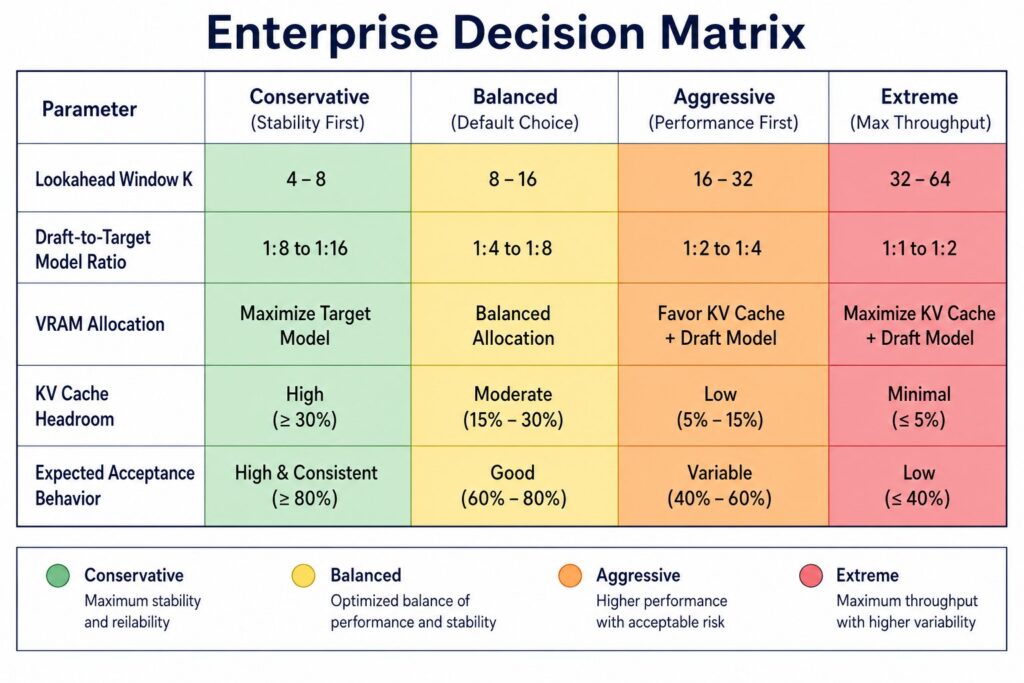
Speculation Tuning Decision Matrix

You should configure your speculation parameters based on your specific hardware profile and model pairing.

The performance tuning parameters include both algorithm-level settings and decoding-specific configurations that determine how aggressively your system speculates.

Your primary tuning vectors are max_depth (controls reasoning step lookahead), width (defines branch expansion in multi-path speculation), num_speculative_tokens (sets token-level draft length), and prompt_lookup_max (limits n-gram matching scope).

Each parameter scales differently with available compute resources.

Your acceptance rate should guide these choices—if it drops below 0.6, reduce your lookahead depth.

Optimizing K Size

The speculation lookahead parameter, commonly denoted as K or gamma, determines how many tokens your draft model generates before verification.

The effectiveness of speculative decoding depends on the speculation lookahead, as values too small trigger excessive target model forward passes while values too large waste compute on redundant drafts.

Your optimal K size balances per-token acceptance rate against verification overhead.

With an acceptance rate α, the expected verified tokens per iteration equals (1 – α^(K+1))/(1 – α).

This mathematical relationship shows why K values above 8-10 rarely improve performance even on high-bandwidth GPUs.

You should start with K=4 for general-purpose workloads and adjust based on your observed acceptance rates.

Short-form generation tasks with predictable patterns can handle K=6 or higher.

Complex reasoning tasks with lower acceptance rates perform better with K=2 or K=3 to minimize wasted speculation.

Draft Size Adjustments

Your draft model’s token generation count per speculation round directly affects memory consumption and speculation efficiency.

Larger draft sizes increase the probability of at least partial acceptance but consume more VRAM for key-value caches and intermediate activations.

When using prompt-lookup decoding with n-gram matching, your draft size should align with typical phrase lengths in your domain.

Technical documentation benefits from 6-8 token drafts that capture common terminology patterns.

Conversational outputs work well with 3-5 token drafts matching natural speech rhythms.

Monitor your draft acceptance rate across different draft sizes to find the sweet spot.

If less than 40% of your drafted tokens are accepted, reduce your draft size by 1-2 tokens.

If acceptance exceeds 80%, you have headroom to increase draft size and potentially capture longer valid sequences.

VRAM Allocation Guidance

Speculative decoding requires additional GPU memory for concurrent draft and target model execution, key-value cache expansion, and verification buffers.

Your total VRAM budget must accommodate both models plus their respective KV caches at your maximum batch size.

Allocate approximately 1.2-1.5x the memory footprint of your target model alone when running speculative decoding.

A 7B parameter target model with a 1B parameter draft typically needs 18-22GB on a single GPU for comfortable operation.

You should reserve 2-4GB for KV cache growth based on your maximum sequence lengths.

For multi-GPU deployments, consider splitting the target model across devices while keeping the draft model on a single GPU.

This topology reduces inter-GPU communication overhead and improves speculation latency.

Your batch size may need reduction by 20-40% compared to standard autoregressive inference to accommodate the additional memory overhead.

Optimizing Acceptance Rate for Throughput and Latency

The token acceptance rate directly determines whether your speculative decoding implementation reduces latency or adds overhead to your inference pipeline.

Higher acceptance rates translate to more verified tokens per speculation round, while rates below certain thresholds can make speculation counterproductive compared to standard autoregressive generation.

Implications of 50% Acceptance

At 50% acceptance, your draft model correctly predicts only half of the proposed tokens on average.

This represents a marginal improvement threshold where speculative decoding may not always yield performance benefits depending on your system load.

With a 50% acceptance rate and a speculation length of 4 tokens, you accept approximately 2 tokens per decoding round.

The target model still performs a full forward pass for verification, consuming compute resources that could otherwise process additional requests in your batch.

Your GPU utilization becomes less efficient because the verification overhead doesn’t justify the modest token gains.

The draft model computation adds latency without sufficient payoff in accepted tokens.

Under high request rates, this acceptance level often increases overall latency rather than reducing it.

Benefits of 70% Acceptance

A 70% acceptance rate represents a practical efficiency point where speculative decoding consistently delivers measurable speedups.

At this level, you accept 2.8 tokens on average from a 4-token speculation window, making the verification overhead worthwhile.

Your inference throughput improves noticeably because the target model generates multiple tokens per forward pass more frequently.

The computational cost of running the draft model and verification becomes justified by the increased output rate.

System performance becomes more stable across varying workloads.

You see consistent latency reductions even under moderate request rates, though performance still degrades under extremely high concurrent loads.

The balance between speculation cost and accepted tokens favors acceleration in most production scenarios.

Achieving 90% Acceptance

At 90% acceptance, your speculative decoding system operates near optimal efficiency.

You accept 3.6 tokens on average from a 4-token window, maximizing the return on verification compute.

Training draft models to directly optimize acceptance rate through specialized loss functions can push performance toward this threshold.

Knowledge distillation techniques that align the draft model distribution with your target model also improve acceptance.

Your latency reductions become substantial, with some implementations achieving 2-3x inference speedup.

The high acceptance rate means nearly every speculation round contributes multiple verified tokens, minimizing wasted computation on rejected candidates.

Effects on Latency and Throughput

Token acceptance rate affects your latency and throughput differently based on system load.

At low concurrency, high acceptance rates directly reduce per-request latency by generating multiple tokens per step.

Under high concurrency with continuous batching, the relationship becomes more complex.

Your batch size grows larger, and speculation can paradoxically increase latency when acceptance rates drop because rejected tokens waste computational resources needed for other batched requests.

Acceptance vs Performance:

The following ranges are illustrative planning assumptions, not guaranteed outcomes; validate them on your own models, hardware, and traffic.

Acceptance Rate	Latency Impact	Throughput Impact	Best Use Case
50%	Minimal to negative	Marginal gain	Low concurrency only
70%	1.5-2x reduction	40-60% increase	Moderate workloads
90%	2-3x reduction	80-120% increase	All workload types

GPU Utilization Considerations

Your GPU utilization patterns change significantly with different acceptance rates.

Low acceptance means frequent rejection of speculated tokens, causing your GPU to perform verification work that produces minimal output.

High acceptance rates maximize useful compute by ensuring most GPU cycles contribute to verified token generation.

You achieve better memory bandwidth utilization because the target model processes longer sequences that yield more accepted tokens.

TensorRT-LLM implementations have demonstrated over 3x speedup in total token throughput on NVIDIA H200 GPUs with optimized acceptance rates.

Your memory pressure also increases with speculation, as you must maintain KV cache entries for both draft and verification phases, making high acceptance rates essential to justify the additional memory overhead.

Medusa Heads vs. Draft Model Speculative Decoding Architecture

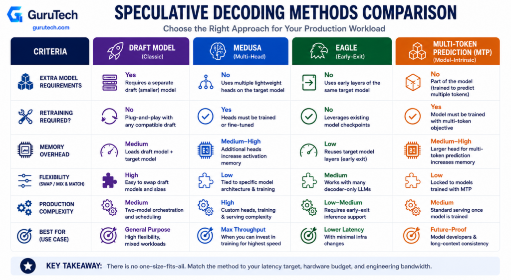
Medusa speculative decoding distinguishes itself from traditional draft model approaches through architectural simplicity and integration efficiency.

Multi-token prediction strategies vary significantly in their implementation overhead, acceptance mechanisms, and suitability for distributed deployments.

Medusa vs Draft Model

Traditional speculative decoding requires you to maintain a separate draft model that generates candidate tokens for verification by your target model.

This approach demands substantial infrastructure overhead since you’re essentially running two models in your serving pipeline.

Medusa eliminates the draft model entirely by adding lightweight prediction heads directly onto your base model.

Each head consists of a single feed-forward layer with residual connections, predicting tokens at different future positions.

You initialize these heads identically to your original language model head, ensuring alignment from the start.

The draft model approach forces you to manage distribution shift between your draft and target models.

Training cost depends on the method, target model, dataset, and number of prediction heads; Medusa-style heads are generally cheaper to train than a full independent draft model.

Medusa avoids this by training heads on top of your existing model representations, maintaining distribution consistency.

Your deployment complexity drops significantly with Medusa.

You don’t need to orchestrate multiple model serving endpoints or handle the intricate scheduling required when coordinating draft and target model calls across distributed systems.

Overview of EAGLE

EAGLE represents an evolution in speculative decoding that builds upon Medusa’s foundation with enhanced prediction mechanisms.

The architecture focuses on improving draft token quality through more sophisticated lookahead strategies.

Unlike Medusa’s parallel prediction heads, EAGLE employs autoregressive generation within the speculation phase itself.

This creates a two-tier autoregressive process where your draft generation is itself autoregressive, then verified by your main model.

EAGLE achieves higher acceptance rates than base Medusa implementations by leveraging richer context during candidate generation.

However, you trade some of Medusa’s simplicity for this improved accuracy.

Your computational overhead increases slightly during the speculation phase, though overall speedups often compensate for this added cost.

The architecture performs particularly well on tasks requiring strong coherence across multiple tokens.

Your acceptance rates improve when generating longer sequences where token dependencies matter significantly.

Introduction to MTP

Multi-token prediction (MTP) approaches train your model to predict multiple future tokens simultaneously during the training phase itself.

You modify your training objective to include auxiliary prediction heads for tokens at positions t+1, t+2, through t+n.

MTP differs fundamentally from Medusa in that you bake multi-token capabilities into your model from the start rather than adding them post-training.

This requires you to commit to the architecture during initial model development, not as a retrofit.

Your MTP heads learn richer representations since they participate in the full training process.

The model develops internal features specifically optimized for predicting future token sequences.

However, you cannot apply MTP to existing pre-trained models without substantial retraining.

The training computational cost increases proportionally with the number of prediction heads you add.

You’re computing loss terms for multiple future positions at every training step, multiplying your gradient computation requirements.

Comprehensive Comparison Table

Architecture	Additional Model Required	Training Requirement	Distributed Serving	Speedup Range	Distribution Alignment
Draft Model	Yes	Pre-train separate model	Complex coordination	1.5-2.5x	Potential shift
Medusa-1	No	Fine-tune heads only	Simple integration	2.2-2.3x	Maintained
Medusa-2	No	Joint fine-tuning	Simple integration	2.3-2.8x	Enhanced
EAGLE	No	Specialized fine-tuning	Moderate complexity	2.5-3.5x	Maintained
MTP	No	Full model retraining	Simple integration	Varies	Native

Your choice depends on whether you’re working with existing models or training from scratch.

Medusa provides 2.2-2.8x speedups while maintaining generation quality, making it practical for retrofitting production models.

EAGLE pushes speedups higher at the cost of implementation complexity.

For existing deployments, you’ll find Medusa-1 offers the fastest path to acceleration since you keep your backbone frozen.

Medusa-2 requires more resources but delivers better performance when you can afford joint training.

Production Deployment Strategies with vLLM

Deploying vLLM in production requires careful configuration of API compatibility layers, parallelism strategies, batching mechanisms, and memory management to achieve optimal throughput and latency for speculative decoding workloads.

OpenAI API Compatibility

vLLM provides native OpenAI API compatibility through its serving layer, allowing you to replace OpenAI endpoints without modifying client code.

You can launch the server with vllm serve <model-name> and immediately expose /v1/completions and /v1/chat/completions endpoints that accept standard OpenAI request formats.

When you enable speculative decoding through vLLM, you pass the configuration via --speculative-config as a JSON object.

Your clients continue using the same API calls while benefiting from reduced inter-token latency.

The server handles all speculation logic transparently.

You should configure health check endpoints at /health and /ready for Kubernetes liveness and readiness probes.

The API compatibility extends to streaming responses, function calling, and logprob returns, ensuring seamless migration from hosted OpenAI services to self-hosted infrastructure.

Implementing Tensor Parallelism

Tensor parallelism splits model weights across multiple GPUs, enabling you to serve models larger than single-GPU memory.

You configure this with --tensor-parallel-size N where N equals the number of GPUs per instance.

For speculative decoding, you must configure both target and draft model parallelism separately.

The draft model typically requires fewer resources, so you can set draft_tensor_parallel_size to a smaller value than your target model’s parallelism degree.

For example, if your target model runs on 4 GPUs, your draft model might only need 1 or 2 GPUs.

Parallelism Configuration Example:

vllm serve Qwen/Qwen3-70B \
  --tensor-parallel-size 4 \
  --speculative-config '{
    "method": "draft_model",
    "model": "Qwen/Qwen3-7B",
    "draft_tensor_parallel_size": 1,
    "num_speculative_tokens": 5
  }'

You should ensure all GPUs within a tensor parallel group have high-bandwidth NVLink or NVSwitch connectivity.

Cross-node tensor parallelism over PCIe or network interconnects introduces substantial latency overhead that degrades speculation efficiency.

Enabling Continuous Batching

Continuous batching allows vLLM to dynamically add new requests to ongoing batches without waiting for all sequences to complete.

This differs from static batching where you must wait for the entire batch to finish before processing new requests.

You don’t need explicit configuration flags to enable continuous batching in vLLM—it operates by default.

The scheduler continuously evaluates incoming requests and available GPU memory to maximize batch utilization.

For speculative decoding workloads, continuous batching becomes more complex because the system must manage both draft and target model forward passes.

Your throughput gains depend on request arrival patterns and sequence length distribution.

Under high QPS scenarios, speculative decoding methods like EAGLE-3 and Medusa maintain medium to high gains even when batches are full, though the relative speedup compared to low-concurrency workloads may decrease.

You can tune max_num_seqs to control maximum concurrent sequences and max_num_batched_tokens to cap total tokens processed per iteration.

Lowering these values reduces memory pressure but may increase queuing latency during traffic spikes.

GPU Memory Management

vLLM uses PagedAttention to manage KV cache memory efficiently, allocating blocks dynamically rather than reserving fixed memory per sequence.

You configure memory allocation with --gpu-memory-utilization, which defaults to 0.90 (90% of available GPU memory).

For vLLM speculative decoding, you need additional memory headroom for draft model weights and intermediate tensors.

If you’re running both models on the same GPU set, you should reduce --gpu-memory-utilization to 0.7-0.8 to prevent out-of-memory errors.

Draft models consume significantly less memory than target models, but speculation increases peak memory usage during verification steps.

Memory Allocation Considerations:

Component	Typical Memory Usage	Configuration Parameter
Target Model Weights	Largest allocation	--model
Draft Model Weights	5-20% of target	speculative_config.model
KV Cache	Dynamic, PagedAttention	--gpu-memory-utilization
Speculation Buffers	~10-15% overhead	num_speculative_tokens

You should monitor GPU memory utilization metrics and adjust gpu_memory_utilization if you observe frequent cache evictions or request rejections.

The max_model_len parameter caps context length and indirectly controls maximum KV cache size per sequence.

Modern vLLM Configurations

Modern vLLM speculative decoding configurations support multiple speculation methods including EAGLE, MTP, draft models, and n-gram approaches.

Your method selection depends on your latency requirements, available GPU memory, and traffic patterns.

For production deployments, you typically choose between model-based methods (EAGLE, draft models) for maximum latency reduction under low-to-medium QPS, or lightweight methods (n-gram, suffix decoding) that maintain gains under high concurrency.

The EAGLE-3 and Medusa methods deliver 2.0-3.2× throughput improvements with bit-exact outputs on the same hardware.

You configure speculation through the --speculative-config JSON object, setting method, model, and num_speculative_tokens as core parameters.

Advanced options include parallel_drafting for EAGLE and draft model methods, rejection_sample_method for controlling verification behavior, and use_heterogeneous_vocab for cross-tokenizer draft models.

Enterprise-Scale Deployment Architecture

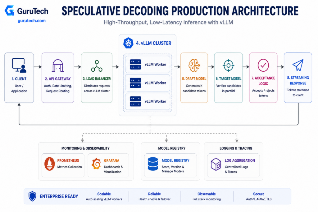
Production deployments require orchestrating draft and target models across distributed infrastructure while maintaining low latency and high throughput.

The architecture must handle request routing, model coordination, observability pipelines, and dynamic scaling to meet enterprise inference throughput demands.

Client to API Gateway Flow

Your client applications send inference requests to an API gateway that serves as the entry point for all traffic.

The gateway handles authentication, rate limiting, and request validation before forwarding payloads to the inference service layer.

This gateway layer typically runs on NGINX, Envoy, or a managed service like AWS API Gateway.

You should configure timeout policies that account for speculative decoding’s variable latency profile, as successful speculation reduces response time while failed drafts may add overhead.

The gateway must parse incoming requests to extract prompt text, generation parameters, and any context metadata.

You route requests based on model version, priority tier, or customer SLA requirements.

Request headers should include tracing IDs that propagate through the entire pipeline for end-to-end observability.

Load Balancing Techniques

Your load balancer distributes incoming requests across multiple inference instances running the target and draft models. Round-robin algorithms work for uniform workloads.

Weighted least-connections performs better when request complexity varies significantly.

You need session affinity when using KV cache warming or stateful request patterns. Consistent hashing ensures that requests with similar prompts land on the same backend instance, improving cache hit rates and reducing redundant computation.

Health checks must verify both model availability and GPU readiness. A simple HTTP 200 response is insufficient because the model might be loaded but the GPU could be experiencing memory pressure.

Your health endpoint should return latency percentiles and queue depth metrics that inform intelligent routing decisions.

vLLM and Draft Model Integration

vLLM serves as the inference engine coordinating both draft and target model execution. You deploy the draft model as a lightweight service that generates candidate tokens before the target model validates them in parallel.

The draft model runs on dedicated GPU instances or shares resources with the target model depending on your memory and compute constraints. Sharing resources reduces infrastructure costs but introduces scheduling complexity that can impact latency.

You configure vLLM to batch draft generation requests and execute target model verification in a single forward pass. The framework handles token acceptance logic, rejection sampling, and KV cache management automatically.

Your configuration specifies the maximum speculation length, typically between 4 and 8 tokens based on your acceptance rate benchmarks.

Advanced deployment patterns include disaggregating the draft and target models across separate infrastructure tiers with different memory and bandwidth characteristics.

Target Model Staging

Your target model runs on high-memory GPU instances optimized for large batch processing and parallel verification. You stage model weights in GPU memory at container startup to avoid cold start penalties during request handling.

Model versioning requires blue-green deployment strategies where new model versions warm up on shadow traffic before receiving production load. You gradually shift traffic percentages while monitoring acceptance rates and output quality metrics.

Weight quantization techniques like FP8 reduce memory footprint and improve throughput without significantly degrading accuracy.

Combining FP8 quantization with speculative decoding enables cost-efficient serving across enterprise workloads.

Your staging pipeline must validate that draft and target model alignment remains high after updates. Mismatched models produce low acceptance rates that eliminate speculation benefits and waste compute resources.

Telemetry for Observability

You instrument the entire pipeline with metrics, traces, and logs that flow into centralized observability platforms like Prometheus, Grafana, or Datadog. Critical metrics include draft acceptance rate, inter-token latency, time to first token, and end-to-end request duration.

Distributed tracing correlates request flow from gateway through draft generation, target verification, and response assembly. Each span captures GPU utilization, memory consumption, and queue wait times at every stage.

Log aggregation captures rejected tokens, speculation failures, and model inference errors that impact output quality. You correlate these events with user-facing latency to identify optimization opportunities.

Industrial-grade monitoring systems track inference acceleration metrics that quantify the speedup ratio between standard autoregressive decoding and speculative approaches.

Autoscaling Considerations

Your autoscaling policies trigger based on GPU utilization, queue depth, and request latency percentiles rather than simple CPU metrics. You set scale-up thresholds at 70% GPU utilization to maintain headroom for traffic spikes.

Horizontal scaling adds inference replicas when queue depth exceeds target thresholds for more than two consecutive minutes. Scale-down policies include stabilization windows that prevent thrashing during variable load patterns.

Draft model instances scale independently from target model infrastructure because their resource profiles differ significantly. Lightweight draft models scale more aggressively to maintain high speculation throughput while expensive target models scale conservatively to control costs.

Predictive autoscaling uses historical traffic patterns to pre-warm instances before expected load increases. You schedule scale-up operations 5-10 minutes before anticipated demand to avoid latency degradation during instance startup.

Complete Response Lifecycle

A request enters through the gateway and lands in the inference queue where it waits for available GPU capacity. The scheduler batches compatible requests together to maximize throughput and hardware utilization.

The draft model generates 4-8 candidate tokens for each queued request. These drafts flow to the target model which processes the original prompt plus all draft tokens in a single forward pass using parallel attention mechanisms.

The target model validates each draft token through rejection sampling, accepting the longest matching prefix. Accepted tokens stream back to the client immediately while rejected positions trigger standard autoregressive generation.

Your response assembly layer formats the output, applies any post-processing filters, and returns the completed text with metadata including token count, latency breakdown, and speculation efficiency.

The lifecycle can complete substantially faster than standard decoding when acceptance is high and scheduling overhead remains controlled.

Observability and Real-Time Metrics

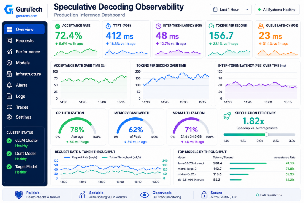
Effective speculative decoding requires continuous monitoring of acceptance rates, latency breakdowns, and resource utilization to validate whether your architecture delivers the expected speedup. You need granular metrics that reveal how draft tokens perform against verification steps and where bottlenecks emerge in your pipeline.

Monitoring Acceptance Rate

Your draft acceptance rate measures the percentage of speculated tokens that pass verification by the target model. This metric directly determines whether speculative decoding provides speedup or adds overhead to your system.

Track acceptance rate per request and across sliding time windows. A rate below 60% typically indicates misalignment between your draft and target models.

You should segment this metric by input length, task type, and user cohort to identify patterns. Low acceptance rates signal that your draft model produces tokens the target model rejects frequently.

This forces the system to fall back to standard autoregressive decoding while still paying the cost of speculation. Calculate acceptance rate as accepted_tokens / total_drafted_tokens and set alerts when it drops below your baseline threshold.

Tracking TTFT

Time to first token (TTFT) represents the latency from request arrival until your system returns the initial token to the user. Speculative decoding can increase TTFT if the drafting phase adds significant overhead before verification begins.

Measure TTFT separately from end-to-end latency to isolate cold-start performance. Your monitoring should capture P50, P95, and P99 percentiles across different request volumes.

High TTFT variance often indicates scheduling inefficiencies or competition for GPU resources during the drafting phase. You need to benchmark TTFT with and without speculative decoding enabled.

If your draft model requires separate GPU allocation or introduces queueing delays, TTFT may degrade even when overall throughput improves.

Analyzing Inter-Token Latency

Inter-token latency measures the time between consecutive token emissions during generation. Speculative decoding aims to reduce this metric by accepting multiple draft tokens in a single verification pass.

Monitor inter-token latency as a time-series metric with millisecond precision. You should calculate mean and variance across generation steps, since early tokens often show different latency characteristics than mid-sequence tokens.

Spikes in inter-token latency reveal when speculation fails and your system reverts to sequential decoding. Compare inter-token latency distributions between standard autoregressive decoding and speculative modes.

Effective implementations show lower mean latency and reduced variance when draft acceptance rates remain high.

GPU Utilization Metrics

GPU utilization reveals whether speculative decoding saturates your compute resources or introduces idle time during draft-verify transitions. You need to track both overall utilization and per-kernel breakdowns to identify inefficiencies.

Monitor GPU memory bandwidth utilization alongside compute utilization.

Memory-bound operations during LLM inference mean that speculation should reduce the frequency of full parameter transfers. If GPU utilization drops below 70% during speculative decoding, you likely have scheduling gaps or poor batching.

Track the ratio of time spent in draft model kernels versus target model verification kernels. Imbalanced ratios indicate that one component dominates your pipeline and limits parallelism gains.

Draft and Verification Latency

You must separate drafting latency from verification latency to understand where your pipeline spends time. Drafting latency includes the time to generate k candidate tokens using your lightweight model, while verification latency covers the target model’s parallel evaluation of those candidates.

Instrument both phases with high-resolution timers. Your draft latency should remain under 20% of the equivalent autoregressive decoding time for k tokens.

Verification latency depends on batch size and sequence length, so track it across different input distributions. Calculate the ratio draft_latency / (verification_latency + draft_latency).

Values above 0.3 suggest your draft model is too slow or your proposal length k is excessive for the available compute.

Tokens Per Second

Tokens per second (TPS) aggregates throughput across all active requests in your system. Speculative decoding should increase TPS when acceptance rates justify the speculation overhead.

Measure TPS at the service level, accounting for all requests in flight. You need to track both raw TPS and effective TPS, where effective TPS only counts accepted tokens.

The gap between these metrics reveals speculation waste.

Key TPS metrics:

Metric	Definition	Target
Raw TPS	All generated tokens / time	Baseline + 30%
Effective TPS	Accepted tokens / time	Baseline + 50%
Speculation overhead	(Raw TPS – Effective TPS) / Raw TPS	< 15%

Queue Latency Assessment

Queue latency measures the time requests spend waiting for GPU resources before execution begins. Speculative decoding can increase queue latency if draft and target models compete for limited resources.

Track queue depth and wait times for both draft and verification operations. Your system should maintain separate queues or use goodput-based scheduling to optimize resource allocation.

Rising queue latency under moderate load indicates insufficient GPU capacity or poor request batching. Monitor the correlation between queue latency and acceptance rate.

When acceptance rates drop, rejected drafts increase queue pressure without delivering throughput gains.

Measuring Speculation Efficiency

Speculation efficiency quantifies the ratio of accepted tokens to total computational cost. You calculate this as (accepted_tokens * target_model_cost) / (draft_cost + verification_cost).

This metric reveals whether your speculation strategy provides net savings. Efficiency above 1.0 means speculation reduces overall compute compared to standard decoding.

Values below 0.8 indicate that speculation overhead exceeds the benefits from parallel verification. Track efficiency across different sequence lengths and request patterns.

Short sequences often show lower efficiency because the fixed cost of initiating speculation dominates. You should disable speculative decoding for requests where predicted efficiency falls below your threshold.

Reference AI Token Observability Dashboard

Your observability dashboard must surface the metrics that indicate whether speculative decoding performs as expected in production.

Build dashboards that combine latency histograms, acceptance rate trends, and resource utilization in a single view.

Include the following panels in your dashboard:

• Acceptance rate time series with P50/P95/P99 breakdowns
• TTFT and inter-token latency distributions
• GPU utilization and memory bandwidth graphs
• TPS comparison between standard and speculative modes
• Queue depth and wait time heatmaps
• Speculation efficiency by request cohort

Configure alerts for acceptance-rate drift, rising inter-token latency, queue growth, and GPU-memory pressure. Correlate those alerts with model versions, prompt-template releases, sampling changes, and autoscaling events so operators can distinguish model-pair degradation from infrastructure contention.

Common Deployment Pitfalls and Performance Tuning

Speculative decoding can reduce inter-token latency substantially, but it is not a universal accelerator. The production result depends on draft quality, request concurrency, sampling settings, context length, GPU topology, scheduler behavior, and the amount of memory remaining for the KV cache. A configuration that performs well in a single-request benchmark may regress under sustained traffic.

Low or Unstable Acceptance Rates

The most common failure mode is a draft model that does not approximate the target model closely enough. Every rejected proposal consumes drafting and verification work without advancing generation. The problem often appears after a target-model update, a prompt-template change, or a shift toward more specialized traffic.

Do not manage acceptance rate as one fleet-wide average. Segment it by task, prompt length, sampling temperature, model version, and customer workload. A general-purpose draft may work well for conversational text but fail on legal, financial, medical, or code-generation prompts.

Excessive Lookahead

A larger lookahead window increases the theoretical number of tokens that can be accepted in one verification pass, but it also increases drafting cost, temporary memory use, and the likelihood that later proposals will be discarded. If a K=8 configuration regularly accepts only two or three tokens, the remaining candidate positions are mostly overhead.

Start with a conservative window such as K=4 or K=5. Increase it only when production telemetry shows consistently high acceptance and sufficient GPU headroom.

GPU Memory Pressure and KV Cache Trade-Offs

Classic draft-model speculation requires memory for two model artifacts, two decoding states, verification buffers, and growing KV caches. Reserving too much VRAM for the draft can force smaller batches, shorter contexts, or more frequent cache eviction. Those losses can outweigh the latency benefit.

Measure peak memory consumption at the longest supported context and highest expected concurrency. Do not size the deployment from model-weight footprints alone.

High-Concurrency and Continuous-Batching Effects

Speculative decoding is often most attractive at low or moderate concurrency, where standard decoding remains strongly memory-bound. At high concurrency, continuous batching may already use the GPU efficiently. Additional drafting and irregular acceptance lengths can complicate scheduling, create padding waste, and increase queue latency.

Evaluate p50, p95, and p99 latency together with aggregate throughput. A lower single-request latency is not a win if queue time rises or total completed requests per second falls.

Tokenizer, Vocabulary, and Model-Version Mismatch

Draft and target models must use compatible tokenization and output vocabularies unless the serving framework explicitly supports heterogeneous vocabularies. Special-token differences, chat-template changes, or mismatched context-position schemes can reduce acceptance or prevent the pair from loading.

Treat the draft-target pair as a versioned production unit. Validate compatibility during CI/CD and repeat acceptance benchmarks whenever either artifact changes.

Unrealistic Benchmarking

Synthetic prompts and short, unconstrained completions can exaggerate speedups. A production benchmark should reproduce actual prompt-length distributions, output lengths, sampling parameters, concurrency levels, hardware topology, and cold-start behavior.

Compare speculative and standard decoding on the same hardware and software version. Record TTFT, inter-token latency, end-to-end latency, accepted tokens per verification pass, effective tokens per second, queue latency, and cost per completed request.

Production Best Practices

1. Establish a baseline first. Measure standard autoregressive serving before enabling speculation so improvements and regressions are attributable.
2. Benchmark several draft candidates. Perplexity alone is insufficient; draft latency and target acceptance matter more directly.
3. Begin with a small lookahead window. K=4 or K=5 is a practical starting point for many workloads, but telemetry should drive the final value.
4. Separate TTFT from decode latency. Speculative decoding primarily targets the decode phase and may not improve prompt prefill.
5. Preserve KV cache headroom. Do not trade away batch capacity or supported context length without measuring the fleet-level consequence.
6. Use canary deployment and feature flags. Route a small percentage of traffic through speculation and retain an immediate fallback to standard decoding.
7. Version draft and target models together. Revalidate tokenizer compatibility, acceptance rate, and latency whenever either model changes.
8. Monitor by workload cohort. Enable or disable speculation dynamically for traffic classes where it produces a measurable benefit.
9. Correlate model and infrastructure telemetry. Acceptance rate, GPU bandwidth, queue depth, and scheduler timing must be visible in the same observability workflow.
10. Optimize the full serving stack. Combine speculation with prompt caching, semantic caching, continuous batching, quantization, and efficient routing rather than treating it as a standalone solution.

Speculative Decoding Architecture: Final Takeaways

Speculative decoding architecture addresses one of the most persistent constraints in large-model serving: autoregressive decoding repeatedly streams a large parameter set through the GPU memory hierarchy to advance generation by only one token. A lightweight draft mechanism changes that economics by proposing several likely continuations that the target model can verify together.

The technique does not make the target model smaller, eliminate HBM pressure, or guarantee a fixed speedup. It amortizes expensive target-model work across accepted candidates. The production benefit therefore depends on how quickly the draft proposes tokens, how often the target accepts them, and whether the serving scheduler can exploit the additional parallelism without sacrificing batch capacity or increasing queue latency.

Classic draft models remain the most portable option for existing checkpoints. Medusa, EAGLE, and native MTP approaches reduce or restructure the drafting overhead but introduce their own training and compatibility requirements. vLLM and other modern inference engines make these methods easier to deploy, yet configuration still requires careful hardware sizing, model-pair validation, and workload-specific benchmarking.

For infrastructure teams, the practical path is incremental: establish an autoregressive baseline, test compatible draft mechanisms, start with a conservative lookahead window, canary the configuration under representative traffic, and monitor acceptance rate alongside TTFT, inter-token latency, throughput, queue latency, and GPU memory pressure.

When those metrics improve together, speculative decoding becomes a powerful component of a layered enterprise inference strategy. When they do not, the correct engineering decision is to reduce speculation depth, change the draft mechanism, or fall back to standard decoding for that workload.

What are your current time-to-first-token, inter-token latency, and acceptance-rate benchmarks? Share your model pair, hardware configuration, or co-location bottleneck in the comments below.

Frequently Asked Questions

What is speculative decoding architecture?

It is an inference architecture in which a fast draft mechanism proposes multiple future tokens and a larger target model verifies those candidates in parallel. The system accepts the longest valid prefix and continues from the first rejected position.

Does speculative decoding change output quality?

Lossless implementations use acceptance and resampling procedures designed to preserve the target model’s output distribution. The draft proposes candidates, but the target model remains authoritative.

Does speculative decoding reduce time to first token?

Its primary benefit is lower decode-phase or inter-token latency. TTFT is dominated by queueing, prompt prefill, model loading, and scheduling, although implementation details can affect it indirectly.

How large should the draft model be?

The best draft is not necessarily the smallest or the most accurate. It must be fast enough to keep drafting overhead low while remaining aligned enough to achieve a useful acceptance rate. A structurally related 1B–8B model is a common starting range for a much larger target, but benchmarking should decide.

What is a good token acceptance rate?

There is no universal threshold. Rates above roughly 60% often indicate useful alignment, but net speedup also depends on draft latency, verification cost, lookahead size, batch behavior, and GPU memory pressure.

How many speculative tokens should be proposed?

Many deployments begin with K=4 or K=5. Smaller windows reduce wasted work when acceptance is low, while larger windows can help predictable workloads with consistently high acceptance.

What is the difference between Medusa and a separate draft model?

A separate draft model is an independent checkpoint that proposes tokens. Medusa adds lightweight future-token prediction heads to the target model, reducing runtime model-hosting overhead but requiring model-specific training.

How does EAGLE differ from Medusa?

EAGLE predicts future hidden features and then derives candidate tokens, which can improve candidate quality and acceptance. It generally requires a compatible trained draft component and deeper integration than a plug-and-play draft model.

Can speculative decoding work with quantized models?

Yes, but quantization changes the baseline latency and memory profile. If a quantized target already decodes quickly, draft overhead may consume a larger share of the total time, so the combined configuration must be benchmarked.

Does speculative decoding help RAG applications?

It can reduce generation latency after retrieval and prompt prefill complete. It does not make vector search or document retrieval faster, so RAG latency should still be measured by stage.

Is speculative decoding useful at high concurrency?

Sometimes, but the benefit often narrows because continuous batching already improves GPU utilization. Irregular acceptance lengths and extra memory use can also increase scheduler and queue overhead.

Which production metrics should be monitored?

Monitor acceptance rate, accepted tokens per verification pass, draft latency, verification latency, TTFT, inter-token latency, end-to-end latency, effective tokens per second, queue latency, GPU utilization, HBM bandwidth, KV cache occupancy, and fallback frequency.