
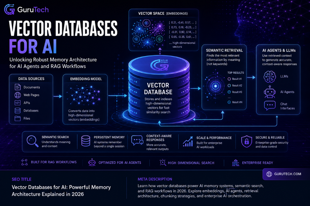
AI applications often stumble in production because they cannot reliably retrieve the right information at the right moment. Large language models process queries in isolation unless someone hooks them up to real knowledge systems.
Vector databases for AI tackle this core problem by giving AI applications persistent, queryable memory—unlocking retrieval augmented generation, semantic search, and context-aware responses that actually tap into real organizational data.
The shift from experimental tools to mission-critical infrastructure for RAG pipelines has made vector databases a must-have for enterprise AI workflows. Modern AI agent memory isn’t just about stretching context windows; it needs purpose-built systems that index high-dimensional embeddings, run similarity searches at scale, and plug right into AI orchestration layers.
Organizations building RAG architecture and semantic search systems have important architectural decisions to make around database selection, deployment models, and workflow design. The wrong choice can reduce performance, increase costs, and create long-term maintenance overhead.
This guide digs into the technical architecture of vector databases, compares leading solutions for different scale needs, and lays out implementation blueprints for production-grade AI memory systems.
Key Takeaways
- Vector databases let AI applications retrieve relevant info using semantic similarity, not just exact keyword matches.
- RAG architecture needs vector storage systems that mesh with embedding models and LLM inference pipelines.
- Choosing between managed and self-hosted vector databases comes down to scale, operational muscle, and budget limits.
Technical Anatomy: How Vector Databases for AI Power Long-Term Memory
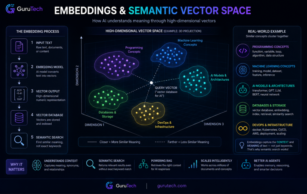
AI systems turn unstructured data into mathematical representations called embeddings—these let machines find semantically similar content by proximity, not just matching keywords. High-dimensional vectors store context and meaning, so AI workflow memory systems can pull up relevant info even when query terms don’t match stored content directly.
Simple but Accurate Embeddings
Vector embeddings transform text, images, or audio into arrays of numbers that capture semantic meaning. Each dimension in these high-dimensional embeddings stands for features that machine learning models extract during encoding.
The AI systems store information as high-dimensional vectors to help models understand meaning and remember context. For instance, a sentence about “banking transactions” might map to a 768-dimensional vector, each position encoding things like financial context, action type, or domain specifics. Similar ideas cluster together in this space.
Embedding models from OpenAI or specialized computer vision services handle the conversion from raw data to these numbers. Both stored documents and user queries need to go through the same embedding model; otherwise, semantic retrieval falls apart. This consistency lets RAG systems match user questions with the right knowledge base entries.
Key embedding characteristics:
| Property | Description | Impact on AI Memory Systems |
|---|---|---|
| Dimensionality | Number of values per vector (384-4096+) | Higher dimensions capture more nuance but eat up storage |
| Cosine similarity | Measures angle between vectors | Shows semantic closeness regardless of size |
| Model consistency | Same encoder for all data | Enables reliable similarity search across documents |
Semantic Chunking Explained
Large documents need to be broken into smaller segments before vector encoding, or retrieval precision declines. Semantic chunking splits content by meaning, not by arbitrary character count.
For example, consider a 10,000-word technical manual—chunking by topic gives more accurate embeddings than just slicing every 500 characters. Each chunk becomes its own vector entry, with metadata pointing back to the source. This avoids the noise that happens when unrelated ideas get squished into a single embedding.
Chunking strategies comparison:
| Method | Chunk Basis | Best For | Limitation |
|---|---|---|---|
| Fixed-size | Character/token count | Simple implementation | Breaks context mid-sentence |
| Sentence-based | Natural breaks | General content | May miss paragraph themes |
| Semantic | Topic boundaries | Technical docs, long articles | Needs preprocessing logic |
| Sliding window | Overlapping segments | Dense information | Uses more storage |
RAG systems usually work best with chunks between 200-800 tokens. Smaller chunks isolate facts for sharper retrieval, while bigger ones keep more context but can muddy search results. Organizations tweak chunk size based on their use cases and query patterns—there’s no one-size-fits-all.
Semantic Proximity Search with Business Examples
Vector similarity search finds entries nearest to a query vector in high-dimensional space. Unlike keyword matching, this semantic search uncovers related content even if the words don’t line up.
If a customer asks “How do I reset my password?”, the system turns that into a vector and searches for the closest support articles. Docs about “account recovery” or “credential restoration” rank higher, even if they never mention “password reset.” The vector search works by performing nearest neighbor searches to retrieve the most similar results.
Approximate nearest neighbor algorithms like HNSW and IVF make fast searches possible across millions of vectors. HNSW builds hierarchical graph structures for a good balance of speed and accuracy. IVF splits the vector space into clusters, so the search only hits relevant areas instead of the whole database.
Search workflow breakdown:
| Stage | Process | Technology |
|---|---|---|
| Query processing | Convert user input to vector | Same embedding model as documents |
| Index traversal | Navigate HNSW graph or IVF clusters | ANN algorithms (FAISS, DiskANN) |
| Candidate selection | Identify top-k nearest vectors | Cosine similarity or Euclidean distance |
| Result ranking | Score by proximity + metadata filters | Hybrid search with vector and keyword signals |
Hybrid search mixes vector similarity and classic keyword filtering. For example, a search for “red leather jacket under $200” uses semantic retrieval for style, but still applies hard filters for color and price. Retrieval augmented generation really shines when you blend semantic understanding with structured constraints.
Enterprise AI orchestration platforms use these vector database operations to power chatbots, recommendation engines, and document analysis tools. The indexing strategy—HNSW for speed, IVF for memory savings—directly shapes query latency and scalability for AI agent memory.
Blueprint: Modern AI Agent Memory Architecture
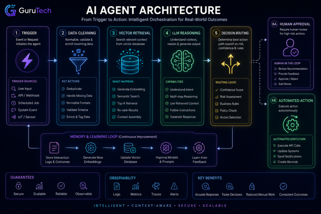
Production AI agents need structured memory systems that split working state from persistent knowledge and decision history. Enterprise RAG setups layer multiple retrieval strategies to keep context sharp across sessions.
Episodic Memory vs Semantic Memory
Episodic memory tracks time-ordered agent decisions, tool calls, and outcomes. This lets agents reconstruct decision chains and spot behavior patterns over time.
Semantic memory holds validated domain knowledge, compliance rules, and factual records that stay stable across agent interactions. Organizations usually keep this in vector databases tuned for similarity search at sub-20ms p99 latency.
| Memory Type | Storage Pattern | Retrieval Method | Typical Backend |
|---|---|---|---|
| Episodic | Time-ordered append | Temporal range filter | Pinecone Serverless |
| Semantic | Validated knowledge | Similarity search | Qdrant with HNSW |
| Working State | Session-scoped | Key-value lookup | Redis OSS |
Keeping these separate stops agents from contaminating ground-truth knowledge with unvalidated, in-progress reasoning. If agents write straight to semantic memory during tasks, the knowledge base degrades over time with noisy outputs.
RAG Retrieval Pipelines in Practice
Retrieval-augmented generation pipelines pull from vector collections before every LLM inference call. The retrieved context supplements the prompt with domain knowledge the model never saw during training.
Production pipelines run pre-filtering on metadata fields before firing off a vector similarity search. This narrows the search space and blocks semantically similar but contextually wrong results from cluttering the prompt.
LangChain and LlamaIndex offer abstractions for multi-stage retrieval, blending dense vector search with keyword matching. Hybrid search boosts recall precision when exact term matches are more important than broad semantic similarity.
Enterprise RAG architectures keep encoding, storage, and retrieval layers separate. Locking the embedding model at the infrastructure level avoids dimensional mismatches between writes and reads.
| Pipeline Stage | Function | Failure Mode |
|---|---|---|
| Query encoding | Convert input to vector | Model version mismatch |
| Pre-filtering | Metadata constraint | Over-filtering returns empty set |
| Vector search | Similarity ranking | Stale embeddings from old model |
| Re-ranking | Score adjustment | Token budget overflow |
Dynamic Context Injection via Vector Retrieval
Vector retrieval picks memories on the fly, based on the agent’s current task state. Instead of loading everything, the system queries for the top-k most relevant vectors that fit within the token budget.
Retrieval confidence scores decide whether content makes it into the prompt. Low-confidence matches get filtered out to keep noise from wrecking reasoning quality.
Deploying agentic AI systems means using temporal weighting strategies. These favor recent memories for time-sensitive tasks but still keep access to historical knowledge. The retrieval layer applies decay functions to similarity scores based on memory age.
Context assembly ranks retrieved memories by relevance, deduplicates overlapping content, and trims the list to fit inside the model’s context window. This keeps token overflow from silently dropping critical context at the end of the prompt.
MCP and Orchestration Layer Considerations
The Model Context Protocol standardizes how agents tap into external data sources and tools during execution. Memory architecture ties in with MCP by exposing retrieval endpoints as callable functions.
Orchestration layers juggle multiple retrieval calls across different memory types in a single agent decision cycle. The orchestrator figures out which memory collections to query, depending on the current task phase.
AI workflow memory management splits hot state—data agents access frequently—from cold storage for historical records. The orchestration layer routes queries to the right backend, balancing latency needs and access patterns.
Function schema registries stored in hybrid vector databases help prevent API hallucination by enforcing exact matches on parameter names and types. BM25 keyword search, combined with semantic embeddings, sharpens retrieval accuracy for structured tool specs.
Cloud vs Self-Hosted Vector Databases
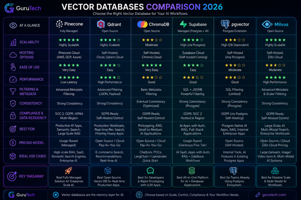
Organizations rolling out RAG architecture and semantic search have to pick between managed cloud services and self-hosted deployments. Each path brings its own trade-offs in operational control, cost predictability, and integration complexity—choices that shape AI agent memory performance and enterprise AI workflows in real, sometimes unexpected ways.
Pinecone
Pinecone runs as a managed vector database service only—there’s no self-hosted flavor. The platform hides all the infrastructure stuff, so you don’t have to worry about indexing, replication, or scaling; it just handles those behind the scenes across its cloud setup.
Organizations get serverless vector search, available through pod-based or serverless deployment models. The serverless tier bills you for storage and read/write operations, which makes sense for RAG workloads that fluctuate.
Pod-based deployments mean you get dedicated compute and predictable pricing, but you’ll need to plan capacity. Pinecone supports metadata filtering, hybrid search, and namespace isolation for multi-tenant apps.
You integrate using REST APIs and client libraries for Python, JavaScript, and a handful of other languages. The platform bakes in monitoring and takes care of index optimization without manual intervention.
But, if an organization needs self-hosting for strict data residency or to avoid vendor lock-in, Pinecone is not the right fit.
Qdrant
Qdrant offers both managed cloud and open-source self-hosted options. You can run the self-hosted version as a single binary or Docker container, and it’s has full feature parity with the managed service.
That means you control where your data lives, how your network is set up, and when or how you scale. Choosing between managed and self-hosted Qdrant comes down to your team’s infrastructure maturity and compliance needs.
The managed side handles updates, backups, cluster management, and delivers SOC 2 Type II compliance. Self-hosted deployments let you plug into your own VPC, set custom security policies, and tap into direct GPU acceleration for embedding generation.
Qdrant uses quantization and on-disk storage options to lower memory demands for large-scale AI embeddings. Distributed deployments use sharding and replication, so you can scale horizontally across nodes.
ChromaDB
Chroma is mainly an open-source vector database that’s meant to be embedded right in your app. By default, it runs in-memory or persists to local disk, which is handy for dev environments or smaller AI memory systems.
If you need to share access across multiple services, you can run Chroma in client-server mode. The architecture is all about developer experience—minimal config, minimal operational friction.
Python and JavaScript clients connect directly to Chroma, so there’s not much setup. This makes it great for prototyping semantic search or RAG architectures fast.
But Chroma doesn’t do native clustering, so distributed deployments aren’t really an option. Managed hosting is pretty limited compared to what you get with enterprise platforms.
Once you need low-latency search at scale, teams often move to a production-grade system after starting out with Chroma.
Supabase
Supabase brings pgvector into PostgreSQL via its managed platform. You get relational database features plus vector similarity search in one package.
Authentication, real-time subscriptions, and storage all come bundled alongside vector operations. Deployments happen on Supabase’s cloud, with automatic backups and point-in-time recovery baked in.
The platform handles PostgreSQL upgrades and security patches, keeping pgvector extension compatibility intact. Pricing scales up with your database size, compute, and data transfer.
If you want to self-host, you’ll need to spin up PostgreSQL, authentication servers, and API gateways yourself. That’s more operational overhead than just deploying a standalone vector DB.
If an organization already uses Supabase, you get consolidated tooling. But if vector search is the primary requirement, specialized systems are usually more efficient.
pgvector
The pgvector extension lets you turn existing PostgreSQL installs into vector-capable databases. If a team already runs PostgreSQL in production, you can add vector search without migrating to something new.
The extension supports exact and approximate nearest neighbor search using HNSW and IVFFlat indexes.
Self-hosted deployment considerations:
- You’ll need PostgreSQL 11 or higher and the ability to install extensions
- Performance depends on your PostgreSQL config and how much memory you’ve has
- It works with your existing backup, replication, and monitoring tools
- But you’re limited to single-server PostgreSQL—no distributed architecture
Managed PostgreSQL services (AWS RDS, Google Cloud SQL, Azure Database) support pgvector too. Those platforms handle the database, but you’ll still need to tune the vector-specific stuff yourself.
At scale, performance falls off compared to purpose-built vector databases. But pgvector is a solid pick if you want operational simplicity over max vector search speed, especially for AI orchestration that needs both structured data and vector embeddings in the same transaction.
Milvus
Milvus gives you a lot of deployment flexibility. It’s open source and you can use the managed cloud version via Zilliz.
You can self-host Milvus on Kubernetes, Docker Compose, or even bare metal. The system splits compute and storage so you can scale each independently.
For development, you can run Milvus in standalone mode. For production, clustered configs span query nodes, data nodes, and index nodes across machines.
This separation lets you scale out to billions of vectors. Here’s a quick breakdown:
| Deployment Mode | Use Case | Infrastructure Requirements |
|---|---|---|
| Standalone | Development, small datasets | Single server, 8GB+ RAM |
| Cluster | Production, billions of vectors | Kubernetes, distributed storage |
| Zilliz Cloud | Managed service | Cloud account, API access |
Milvus integrates with MinIO, S3, and Azure Blob Storage for persistent storage. GPU acceleration boosts index building and search speed—crucial for enterprise AI workflows where latency matters.
The system supports HNSW, IVF, and DiskANN indexes for different latency-throughput trade-offs.
Scalability
Horizontal scalability is the big question: can your vector database keep up as AI agent memory grows, without dragging down performance?
Managed services hide scaling complexity with automatic resource provisioning. If you’re self-hosting, you’ll need to configure clusters yourself.
Purpose-built vector databases like Milvus and Weaviate use sharding to split vectors across nodes. Each shard manages a chunk of the dataset, so queries can run in parallel.
Qdrant supports collection sharding with configurable replication for high availability. PostgreSQL-based solutions (pgvector, Supabase) mostly rely on vertical scaling or read replicas to grow.
But once you hit billions of vectors, those approaches hit a wall. Specialized systems just outperform them. If you’re planning RAG at scale, you really need to look at distributed architecture support before picking your platform.
Scaling comparison across deployment models:
| Platform | Deployment | Best For | Main Strength | Main Weakness |
|---|---|---|---|---|
| Pinecone | Managed cloud | Enterprise RAG systems | Operational simplicity and serverless scaling | Vendor lock-in and limited self-hosting control |
| Qdrant | Managed cloud or self-hosted | Flexible AI memory deployments | Strong filtering, performance, and deployment choice | Requires tuning for larger self-hosted clusters |
| ChromaDB | Local/open-source | Development, prototyping, and smaller apps | Simple setup and fast experimentation | Limited large-scale clustering features |
| Supabase | Managed PostgreSQL with pgvector | Full-stack apps already using Supabase | Unified database, auth, storage, and API layer | Less optimized than specialized vector databases at high scale |
| pgvector | PostgreSQL extension | Teams already running PostgreSQL | Easy integration with existing relational data | Scaling limits compared with purpose-built vector systems |
| Milvus | Self-hosted or Zilliz Cloud | Massive vector datasets and high-throughput retrieval | Distributed scalability and advanced indexing options | Higher operational complexity |
Step-by-Step RAG Workflow Logic
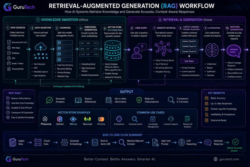
RAG architecture changes the way systems retrieve and generate responses by blending vector search with language models. The workflow runs from document prep to embedding storage to final response synthesis, with each phase needing careful decisions about chunking, retrieval, and prompt design.
Data Ingestion
Data ingestion lays the groundwork for RAG by prepping raw documents for vectorization. Systems have to handle all sorts of formats—PDFs, HTML, markdown, plain text, you name it.
The pipeline pulls out text and tries to keep structure like headings, tables, and lists intact. Document loaders parse these formats and spit out standardized text.
At the same time, metadata extraction grabs details like source URLs, creation dates, authors, and doc types. Real-time indexing lets systems process new docs as soon as they land, so knowledge bases stay fresh.
Most teams add filtering rules during ingestion to weed out junk or low-value content, keeping the vector DB clean.
Chunking Strategy
Chunking strategy is a big deal for retrieval quality and context relevance. Fixed-size chunking splits docs by a set number of characters or tokens—usually 256 to 1024 tokens per chunk.
Semantic chunking breaks at paragraph ends, sentence boundaries, or section headers, so you keep context together. That means variable-length segments, but you don’t lose meaning. AI workflows dealing with technical docs usually prefer semantic chunking for this reason.
Recursive chunking goes by hierarchy—first by sections, then subsections, then paragraphs. It’s handy for structured content with clear outlines.
| Chunking Method | Best Use Case | Typical Size |
|---|---|---|
| Fixed-size | Uniform processing requirements | 512 tokens |
| Semantic | Preserving complete thoughts | 200-800 tokens |
| Recursive | Hierarchical documents | Variable |
| Sentence-based | High precision requirements | 50-200 tokens |
Overlap Windows
Overlap windows help prevent info loss at chunk edges by sharing content between neighboring chunks. For example, a 50-token overlap keeps concepts split across boundaries retrievable.
Higher overlap means more storage, but you get better retrieval completeness. Most systems use 10-20% overlap, but technical docs sometimes need 25-30% to catch complex ideas that span sentences.
The overlap strategy impacts both storage costs and query speed. More overlap means more vectors, but less risk of missing context.
Embedding Generation
Embedding generation turns text chunks into high-dimensional vectors that capture semantic meaning. Models like sentence-transformers, OpenAI’s text-embedding-3, or Cohere’s embed-v3 handle this job.
Model choice changes vector dimensionality—could be 384 for light models, up to 1536 or 3072 for heavyweights. More dimensions mean richer semantics but higher storage and compute costs.
Batch processing helps—convert lots of chunks at once. GPU acceleration seriously cuts down processing time for big document sets.
It’s always a trade-off: model power versus infrastructure cost. Choose carefully.
| Model Family | Dimensions | Performance | Use Case |
|---|---|---|---|
| MiniLM | 384 | Fast, lightweight | High-volume applications |
| BERT-based | 768 | Balanced | General semantic search |
| OpenAI Ada | 1536 | High accuracy | Enterprise applications |
| Cohere v3 | 1024-4096 | Customizable | Multi-language systems |
Retrieval Querying
Retrieval querying works by turning user questions into vectors, then running similarity searches against the vector DB. The query encoder needs to match the embedding model you used for indexing—otherwise, vectors won’t line up.
Approximate nearest neighbor algorithms keep retrieval fast, even with millions of vectors. Cosine similarity is the go-to metric for text, but you’ll also see Euclidean distance or dot product.
Top-k retrieval grabs the k most relevant chunks—usually between 3 and 10. More context means longer prompts and higher costs, so there’s always a balancing act.
Hybrid search blends vector similarity with keyword matching for better accuracy on exact terms or names. Metadata filtering lets you narrow results by date, doc type, or category before or after the vector search.
Prompt Injection
Prompt injection is where you combine retrieved context with the user’s query to build the final input for the language model. The template you use here really matters for both quality and sticking to the facts.
Usually, you include system instructions, the most relevant retrieved chunks, and the user’s question. Most systems order context by similarity score—most relevant first. Sometimes, you’ll add metadata like source docs or page numbers for citations.
Context Ordering Strategies:
- Relevance-first: Highest similarity scores come first
- Chronological: Order by time for temporal questions
- Source-grouped: Cluster chunks from the same doc together
- Interleaved: Mix chunks from different sources for balance
You have to watch your token budget—keep the prompt under model limits while saving room for the answer. Truncation strategies chop off lower-relevance chunks when you get close to the cap.
Reasoning Layer
The reasoning layer runs queries and context through the language model. At this point, AI orchestration decides how the model interprets what it retrieves and crafts a response.
Temperature settings play a big role here. Lower values (0.1–0.3) keep outputs consistent and focused on facts, which is usually what you want in RAG setups.
Higher temperatures? Sure, you get more creativity, but you also crank up the risk of hallucinations.
Chain-of-thought prompting nudges models to show their work—reasoning steps come before final answers. This helps a lot when queries require multi-step logic, not just a quick lookup.
The reasoning layer sometimes adds verification by cross-referencing generated content against what was actually retrieved.
Some teams use multiple LLM calls: one to refine the query, one to generate an answer, and maybe a third for fact-checking. Yes, this adds latency, but the bump in accuracy can be worth it.
Response Generation
Response generation pulls the final answer together from the model’s output, staying grounded in the retrieved context. Streaming responses send tokens as they’re ready, which helps with perceived speed, especially for longer answers.
Citation systems track which chunks informed which parts of the response. Inline references or footnotes let users check sources on the fly.
AI agent memory systems might log generated responses for future review or quality checks. Output formatting—markdown, bullets, or structured data—makes everything easier to scan and use.
Why Bigger Context Windows Are NOT Real Memory
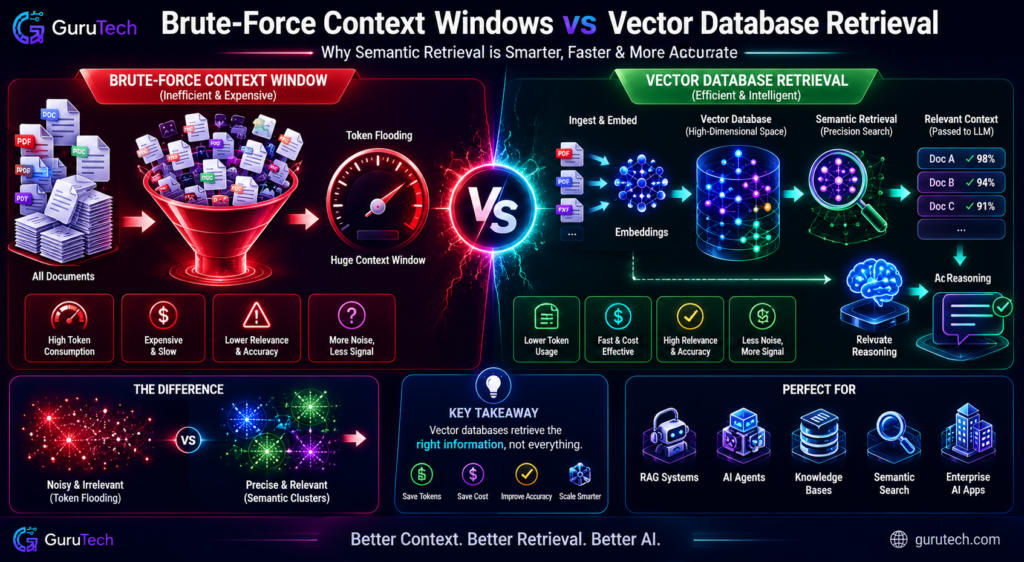
Expanding context windows to 128K, 200K, or even 1M tokens looks like persistent memory, but under the hood, the architecture treats every interaction as a static input. These giant windows introduce computational bottlenecks and degrade accuracy—problems vector database architectures sidestep by design.
Token Flooding
Massive context windows force models to chew through thousands of tokens, relevant or not. If you dump a 100K token conversation history into every request, the model has to sift through everything—promos, confirmations, tangents, and the crucial business logic—all at once.
This creates information density headaches. RAG solves this by pulling just the 5–10 most relevant chunks, not the entire conversation log.
Token Processing Comparison:
| Approach | Tokens Processed | Relevant Information |
|---|---|---|
| Large Context Window | 100,000+ | 2-5% |
| Vector Database Retrieval | 2,000-5,000 | 85-95% |
Enterprise AI workflows get more from precision than sheer volume. Retrieval augmented generation pinpoints which customer patterns matter right now, rather than dumping all history into the mix.
Attention Dilution
The attention mechanism’s quadratic scaling means computational complexity goes wild as token counts grow. At 32K tokens, you’re looking at a billion attention entries. At 100K, you hit 10 billion.
Signal-to-noise tanks as attention spreads over huge token sequences. Details buried at position 47,000 have to fight with filler at 89,000. The softmax distribution flattens, and important info just gets lost.
AI agent memory systems handle this with hierarchical storage. Short-term context keeps the immediate state; vector databases hang onto historical patterns for semantic search. This split keeps attention mechanisms from drowning in noise.
Latency and API Costs
Processing 100K tokens per request cranks up infrastructure costs and slows responses. API pricing scales with tokens, so context-heavy designs can blow up your budget fast.
Cost Structure Analysis:
| Architecture | Tokens Per Request | Monthly Cost (10K requests) |
|---|---|---|
| Full Context Window | 95,000 | $4,750 |
| RAG + Vector DB | 8,000 | $400 |
| Hybrid Memory System | 12,000 | $600 |
Latency takes a hit, too. A 128K token prompt can take 3–8 seconds, while targeted retrieval with 8K tokens wraps up in under a second. Strategies to reduce AI API costs focus on cutting redundant token processing with semantic workflows.
AI embeddings—vector representations—compress meaning into 1,536-dimensional arrays. Comparing embeddings? Milliseconds. Reprocessing 100K tokens? Seconds, easily.
Hallucination Amplification
Big context windows make it easier for models to get confused or just make stuff up. When models scan 200K tokens without strong relevance signals, they start stitching together unrelated info.
AI memory systems score confidence on retrieved chunks. If similarity falls below 0.7, the system admits it doesn’t know, instead of inventing answers from weak context.
Hallucination Risk Factors:
- Context length >64K tokens: Accuracy drops 15–30%
- Mixed domains: Models blend unrelated topics
- Temporal confusion: Recent and historical data blur together
AI orchestration sets up guardrails large context windows just can’t. Metadata tags, timestamp filters, and source attribution help build a verifiable chain of information.
Retrieval Precision vs Brute-Force Prompting
Semantic search turns natural language queries into vectors, then finds the top-k nearest neighbors in embedding space. This is way more precise than keyword matching or brute-forcing context windows.
Say a customer asks about “refund processing delays.” The system grabs policy docs, past escalations, and workflows. Brute-force context just dumps every customer interaction, forcing the model to guess what matters.
Retrieval Workflow Logic:
| Step | Vector Database | Context Window |
|---|---|---|
| Query Processing | Embed user question (0.05s) | Load full history (2.3s) |
| Relevance Filtering | Cosine similarity >0.75 | No filtering |
| Context Injection | 4-6 targeted chunks | 50K+ mixed tokens |
| Response Generation | High precision (0.8s) | Low precision (3.1s) |
Enterprise AI workflows need audit trails showing which knowledge drove each decision. Vector database guides track chunk IDs, similarity scores, and timestamps. Context windows? That visibility is limited—the model eats everything, and you can’t say what informed the answer.
Common RAG Architecture Mistakes
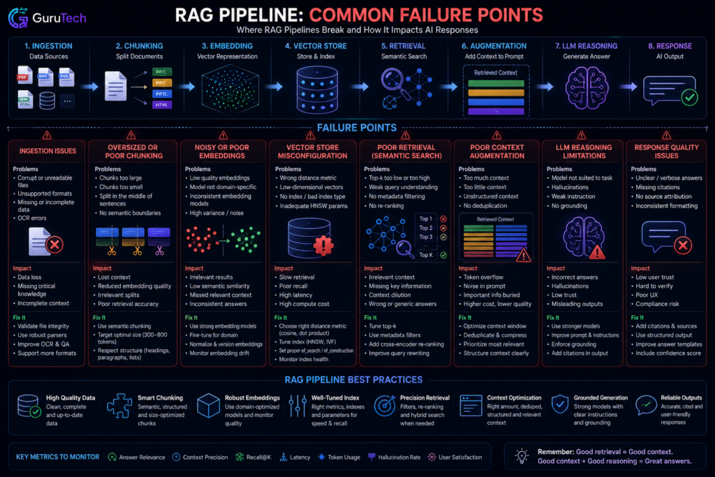
Most production RAG failures come from data prep errors and retrieval pipeline missteps—not model choices. Teams often obsess over embedding models and vector similarity, but overlook how chunking, metadata, and filtering actually control whether the AI agent memory surfaces the right context.
Oversized Chunks
Chunk size is a huge factor in semantic search pipelines. Teams often default to 1000–2000 character chunks without thinking through the impact on context quality.
Large chunks cause headaches. The embedding is just an average of everything in the chunk, which dilutes the signal for focused queries. If someone asks about a specific contract clause buried in a 2000-character chunk, the similarity score reflects the whole blob, not the key sentence.
Optimal chunk sizing varies by content type:
| Content Type | Recommended Size | Reasoning |
|---|---|---|
| Technical documentation | 200-400 characters | Focused concepts, code examples |
| Legal contracts | 300-600 characters | Clause-level granularity |
| Marketing content | 400-800 characters | Paragraph-level ideas |
| Chat transcripts | 100-300 characters | Individual exchanges |
Oversized chunks also burn through your token budget fast. If RAG pulls three 2000-character chunks, that’s 6000 characters in your context window when 600 would’ve worked with better chunking.
Poor Metadata Practices
Metadata filtering separates solid RAG systems from those that leak data across org boundaries. The first RAG deployment almost always uses a single shared workspace—no tags, no separation—which creates compliance risks when HR docs show up in engineering queries.
Every chunk needs filterable metadata fields that match your access controls. Basic setups just store the source doc ID. In production, you need workspace IDs, classification tags, creation dates, and author info.
Essential metadata fields for enterprise AI workflows:
- Workspace/tenant ID – Mandatory for multi-tenant setups
- Security classification – Lets you filter before retrieval
- Document type – Routes queries by content
- Last updated timestamp – Supports time-aware retrieval
- Author/department – Enables role-based filtering
Filter metadata at the vector DB query stage, not after. This way, unauthorized content never even gets embedded. If you filter post-retrieval, you’re just wasting compute on stuff that should’ve been excluded from the start.
Storing Noisy Documents
Vector databases keep whatever quality you feed them. Teams often ingest raw HTML, noisey PDF exports, or boilerplate-laden docs without any cleanup.
This noise pollutes your semantic index. A chunk like “Page 47 of 203 | Company Confidential | Do Not Distribute” plus a couple real sentences leads to an embedding that’s mostly boilerplate. The RAG system then surfaces these junk chunks for queries matching common footer text.
Document preprocessing should strip out:
- Navigation menus and site chrome
- Repeated headers and footers
- Auto-generated metadata blocks
- PDF extraction artifacts
- Empty or near-empty sections
Tables need special treatment. If you store raw table HTML, you just get embeddings of markup. It’s better to extract table data into structured metadata or generate natural language summaries of what’s in the table.
Retrieving Too Many Snippets
Top-k retrieval settings decide how many chunks the RAG architecture hands off to the language model. Common retrieval-augmented generation mistakes often crop up when teams just set k=10 or k=20 by default, without actually checking if it helps answer quality.
Piling up too many retrieved snippets hurts performance in a couple of ways. It eats up precious context window space with barely relevant chunks, making it harder for the model to focus on what matters most.
It also slows things down—more chunks mean the model has to chew through thousands of extra tokens. That’s a quick way to introduce latency.
| Retrieved Chunks | Avg Latency | Context Utilization | Answer Quality |
|---|---|---|---|
| k=3 | 1.2s | 35% | Baseline |
| k=5 | 1.8s | 58% | +12% |
| k=10 | 2.9s | 89% | +8% |
| k=20 | 4.7s | 98% | -3% |
The link between k and answer quality isn’t linear. Quality tends to flatten out—or even drop—once you’re past whatever the sweet spot is for your use case.
In enterprise AI workflows, it’s much smarter to adapt k dynamically, maybe using query confidence scores, instead of sticking to a fixed number.
Adding a re-ranker stage helps: pull k=20 candidates from the vector database, then let a heavier cross-encoder model pick the top 3-5. You get broad recall, sharp ranking, and keep the context size manageable. It’s a premium work, but worth it.
Embedding Low-Quality Data
The AI orchestration pipeline pretty much inherits whatever data quality issues exist upstream. Teams sometimes embed documents without checking if the content is even complete, accurate, or remotely relevant to expected queries.
Some classic quality pitfalls? Only uploading the first page of a contract, outdated policy docs that contradict current procedures, or duplicates hiding under slightly different filenames. The vector database stores all of this the same way, so the AI memory might surface the wrong version or incomplete context.
Data quality gates before embedding:
- Completeness validation – Check page counts, look for all required sections
- Deduplication – Use hash-based matching across your sources
- Recency checks – Flag or skip superseded versions
- Content validation – Enforce a minimum word count, detect language
- Format verification – Make sure text extraction actually works
Teams should add quality scoring to ingestion. Anything below the threshold gets quarantined for manual review instead of going straight into the vector database. That’s how you avoid the classic “poor input quality produces poor AI memory performance” trap in AI memory systems.
Missing Filtering Layers
Production RAG systems really need multiple filtering layers beyond just vector similarity. Teams new to this space often lean entirely on embedding-based retrieval and forget to think about where filtering should actually happen.
Put metadata filtering right inside the vector database query, not as an afterthought. That way, the database can skip irrelevant chunks before it even starts the heavy similarity calculations.
If you filter a query to workspace=engineering, there’s no reason to compute distances for everything else. Save the compute for what matters.
Conclusion: AI Memory Is a Data Architecture Problem
Vector databases are not just another storage option for AI projects. They are the memory layer that lets AI agents retrieve the right knowledge at the right time without flooding every prompt with irrelevant context.
For small experiments, a long prompt or local prototype may be enough. For production systems, the real advantage comes from clean ingestion, strong metadata, precise chunking, reliable retrieval, and an orchestration layer that knows when to query memory before asking the model to reason.
The future of enterprise AI will not be determined only by larger context windows or better prompt templates. It will depend on how effectively organizations structure, retrieve, and govern knowledge across distributed memory systems.
Frequently Asked Questions
Vector databases always spark a bunch of technical questions—implementation details, architecture tradeoffs, operational headaches. Getting a handle on vector representations, similarity metrics, database selection, and what actually works in production can make or break your AI system.
What is a vector in the context of a vector database?
A vector here means a numerical array—coordinates in high-dimensional space. Embeddings usually have hundreds or thousands of floating-point numbers, all generated by machine learning models.
Text embedding models turn sentences into vectors, so that semantically similar stuff lands close together in vector space. For example, “automobile repair” and “car maintenance” produce vectors that sit near each other, even if they don’t share any actual words.
Dimensionality depends on the model. OpenAI’s text-embedding-3-small spits out 1,536-dimensional vectors, while text-embedding-3-large goes up to 3,072. Image models like CLIP? They use different sizes, tuned for visual similarity.
Each dimension encodes some abstract feature the model learned during training. These features let AI agent memory systems retrieve contextually relevant info, way beyond just matching keywords.
How do vector databases enable semantic search and similarity matching?
Vector databases work by mapping data points into a continuous geometric space and then calculating distances between query vectors and stored vectors. This lets you find conceptually related content, not just exact text matches.
It starts when embedding models convert stored docs and queries into vectors. The database then runs similarity metrics to find the closest matches.
Three main metrics measure vector similarity:
| Metric | Calculation Method | Best Use Case |
|---|---|---|
| Cosine similarity | Angle between vectors, ignores magnitude | Text embeddings, semantic search |
| Euclidean distance | Straight-line distance in vector space | Image embeddings, spatial data |
| Dot product | Vector multiplication for normalized vectors | Fast computation when vectors are pre-normalized |
Most RAG implementations stick with cosine similarity, since text embedding models are built for angular distance. Always match your metric to how the embedding model was trained.
Advanced setups mix vector similarity with metadata filtering. Say a user searches product docs—they might want only a specific version or department, so the database has to filter by attributes before or after running vector distances.
What are the key features to evaluate when selecting a vector database for production use?
For production, you’ve has to look at indexing algorithms, filtering, latency, and operational models. These choices hit workflow memory performance and your long-term infrastructure spend.
Pick your indexing algorithm wisely. HNSW (Hierarchical Navigable Small World) usually gives the best speed/accuracy tradeoff—logarithmic search time, high accuracy. IVF (Inverted File Index) is better if you update data a lot, but you’ll lose some precision.
Filtering complexity matters, especially in enterprise AI. Simple category or date filters work everywhere, but complex nested filters need a robust engine. Hybrid search (vector plus keyword) is essential for RAG systems.
Scale changes everything:
| Vector Count | Recommended Approach | Latency Expectations |
|---|---|---|
| Under 1 million | PostgreSQL with pgvector or lightweight options | 50-200ms |
| 1-100 million | Purpose-built vector databases | 20-100ms |
| Over 100 million | Distributed systems or enterprise tiers | Needs careful tuning |
Operational model depends on your team. Managed services take the ops burden off your plate, but you’ll pay more per query. Self-hosted gives you control and cost savings at scale, but now you’re on the hook for database admin.
Which vector databases are most commonly used in enterprise applications today?
Enterprise teams focus on purpose-built vector databases, traditional database extensions, and integrations from cloud providers. Each path fits different operational needs and scales—there’s no one-size-fits-all here.
Pinecone is widely used in managed vector database deployments. Its operational simplicity and hybrid search features make it a top pick when organizations want to keep infrastructure headaches to a minimum, even if it means paying a premium.
Weaviate and Qdrant stand out in the self-hosted world. Weaviate’s has built-in vectorization and GraphQL APIs, which feels pretty developer-friendly. Qdrant, built in Rust, delivers fast performance and advanced filtering—great for teams chasing speed and precision.
PostgreSQL with the pgvector extension is common among teams that already run Postgres. This route works especially well for AI embeddings workflows at smaller scales, letting teams avoid spinning up brand-new database systems just for vectors.
The comparison of commonly used vector databases highlights some clear tradeoffs:
| Database | Deployment Model | Primary Strength | Typical Enterprise Use |
|---|---|---|---|
| Pinecone | Managed only | Minimal operational overhead | Rapid AI orchestration deployment |
| Weaviate | Both managed and self-hosted | Built-in vectorization and flexible APIs | Custom enterprise AI workflows |
| Qdrant | Both managed and self-hosted | Performance and filtering complexity | High-throughput semantic search |
| Milvus | Self-hosted with Zilliz Cloud | Massive scale handling | Large-scale recommendation systems |
| pgvector | Self-hosted extension | Integration with existing Postgres | Incremental AI memory systems adoption |
Cloud providers bring their own flavor to the mix. AWS OpenSearch, Azure AI Search, and Google Vertex AI Vector Search offer tight links to their respective AI stacks, but honestly, you’re trading flexibility for convenience—and picking up some vendor lock-in along the way.
What are practical examples of using a vector database in an AI application workflow?
Vector databases drive a bunch of patterns—AI agent memory, document retrieval, recommendation systems. The details change from project to project, but the architectural backbone is usually pretty similar.
RAG architecture (Retrieval-Augmented Generation) probably tops the list for real-world use. Here, you store document chunks as embeddings, then pull relevant sections based on user queries to give your language model something solid to work with.
Say you’re building a customer support tool. You might index thousands of help docs, letting the AI pull up exactly what it needs to answer a question—no more vague answers, just targeted references.
Semantic search is another area where vector databases shine. Instead of keyword matching, you’re finding content by actual meaning.
Picture an e-commerce site: a search for “comfortable walking shoes” surfaces products described as “cushioned sneakers for daily wear” because, in vector space, those ideas sit right next to each other. That’s a game-changer for user experience.
Here’s a typical AI workflow memory pattern, laid out step by step:
| Stage | Process | Vector Database Role |
|---|---|---|
| Ingestion | Documents chunked and embedded | Store embeddings with metadata |
| Query Processing | User question converted to vector | Accept query vector |
| Retrieval | Similarity calculation performed | Return top-k nearest neighbors |
| Context Assembly | Retrieved chunks formatted | Provide source documents |
| Generation | LLM generates response | Supply semantic context |
Recommendation engines? They lean on vector similarity too.